Wastewater treatment plants (WWTPs) are facing growing pressure to become more efficient and environmentally friendly. WWTPs adopting ProcessMiner’s advanced AI technology are making great progress in optimizing their operations. By taking advantage of ProcessMiner’s advanced AI technology, WWTPs are able to automate critical activities, use resources more efficiently, and reduce their environmental impact. AI also enables the optimization of chemistry and energy consumption in clarifiers, aeration basins, anaerobic /aerobic digesters, and the sludge dewatering process.
Addressing the Challenges WWTPs Face
WWTP operators and environmental engineers often grapple with significant challenges managing operational efficiency and meeting effluent quality limits. Challenges also include:
Handling increasing amounts of contaminants
Reducing the environmental impact of sludge disposal
Optimizing the use of chemicals
Using energy more efficiently
Executing corrective actions in a timely manner
Reducing human error
The ability to address these obstacles directly contributes to operational cost management and environmental impact, which can threaten economic viability and environmental responsibility. While there are several strategies to help address these challenges, one key strategy is automating the optimization of polymer dosing, which is critical to the sludge dewatering process.
The execution of an optimized polymer dosing strategy can lead to significant improvements. Today, we know up to 40% of the cost of water treatment is associated with sludge dewatering. Therefore, the ability to dose the optimum amount of polymer supports the production of a drier sludge cake, reducing the cost of chemicals and increasing plant efficiency as centrifuges, screw presses, and belt presses operate efficiently and optimally.
How ProcessMiner Optimizes the Wastewater Treatment Process
ProcessMiner’s turnkey solution is specifically designed to automate the sludge dewatering process.
By combining the power of AI with intelligent sensing meters placed at critical points in the dewatering process, the solution works by monitoring constantly changing sludge conditions and precisely adjusting polymer dosage to consistently produce a drier sludge cake.
This transformative approach to wastewater treatment supports timely and precise control setting adjustments to improve the efficiency and effectiveness of the water treatment process. In addition, since the platform runs autonomously, it frees up plant operators to focus on other critical plant activities. Finally, because ProcessMiner is adaptive and self-learning, it requires no staffing of data engineers or scientists to maintain the solution as dynamic conditions in the plant evolve.
The end result? Optimized polymer dosing and reduced energy consumption, all while resulting in lower sludge cake transportation and disposal costs. The integration of traditional water treatment processes and plant domain expertise with this level of advanced technology ensures that WWTPs operate at optimal efficiency with the lowest possible environmental impact.
Request a demo today of what’s now possible with AI.
Challenge: Dealing With Unusually High Defect Rates
A leading plastic injection molding manufacturer was experiencing high defect rates in a medical specialty plastic vial product. The manufacturer solicited the help of ProcessMiner to identify and mitigate the root causes associated with the defect rates.
Solution: Using AI to Find Out Scrap Rate Root Cause
Recognizing the potential to leverage AI for process optimization, together the manufacturer and ProcessMiner collaborated on a pilot project. The primary goal was to assess if ProcessMiner’s AI platform could effectively monitor, predict, and prevent defects that were increasing scrap rates in excess of 20% above the company average.
The project began with an extensive offline data analysis to evaluate the data quality accurately from the pilot machine. This critical step enabled a detailed understanding of essential manufacturing quality parameters and control elements.
Within the first 90 days, ProcessMiner’s AI platform analyzed data from more than 300 sensors on the injection molding machine. This analysis pinpointed two specific defect types responsible for a majority of the scrap in the specialty bottle production.
Using these insights, ProcessMiner’s AI platform provided targeted recommendations for adjusting key parameters such as temperature and pressure settings. These recommendations were crucial for refining production quality.
Results: 6-Figure Savings and Improved Scrap Rate
Implementing ProcessMiner’s AI-driven recommendations reduced scrap rates by 25%, significantly enhancing operational efficiency. The pilot also equipped the manufacturer with advanced tools for real-time monitoring and automated corrective action. These tools facilitated proactive adjustments through prescriptive parameter control recommendations automatically transmitted to the plastic injection machine control systems.
ProcessMiner’s introduction of autonomous control that allowed for automatic adjustments to production set points via IoT technology. This closed-loop system and autonomous control platform streamlined operations, consistently reduced defects, and maximized productivity, resulting in a higher first-pass yield.
Throughout the pilot, ProcessMiner’s AI platform autonomously adjusted the plastic injection molding machine settings at the start of each manufacturing shift. This consistency significantly reduced production variability and increased stability.
By autonomously maintaining optimal machine settings, the platform helped create a more predictable and efficient manufacturing environment, ultimately yielding annualized six-figure operational savings for the company.
Author: Chitta Ranjan, Ph.D., Director of Science, ProcessMiner, Inc.
Industry: Chemicals, Pulp & Paper
Overview
The goal of this project was to autonomously control part of a tissue mill’s continuous manufacturing process using artificial intelligence and predictive analytics to reduce raw material consumption while maintaining the product quality with specification limit.
Predictive analytics uses a manufacturing machine’s historical data to predict process outcomes. Through machine learning and artificial intelligence, these models continue to learn, adapt and evolve, providing the user with accurate information that can drive better decisions.
Challenge
It is difficult to learn a multitude of relationships in a complex manufacturing environment. Typically, an operator uses his or her past experiences in determining how to regulate the dosage of a raw material with:
preferred minimum raw material consumed, while
keeping the product quality within range
The challenge, therein, lies with the operator’s ability to act quickly with the dynamically changing manufacturing processes, and deliver continuous process improvement with autonomous chemistry control.
Solution
This is where the ProcessMiner AutoPilot real-time predictive system comes in and solves the problem, making recommendations and prescribing solutions. In doing this, it minimizes raw materials and reduces costs while maintaining both speed and product quality.
ProcessMiner’s AI platform is a cloud-based system that utilizes information, including:
Physical tissue/papermaker property measurements
Tissue/papermaking process knowledge
System ‘meta-data’ to mathematically model the tissue/papermaker system
The information generated by this continuously-learning model is then used to accurately predict key performance indicators (KPI) of the tissue/paper machine, and therefore, provide actionable insights.
The Solenis OPTIX ProcessMiner AutoPilot platform is designed to be an adaptive and evolving artificial intelligence system, allowing it to automatically and simultaneously learn these relationships. The adaptive analytics system accurately learns complex variable relationships in pulp and paper manufacturing processes and yields a digital measure of product quality.
For example: every time the system hits a new data point, it runs an orchestration (sequence of steps) series of processes, and in turn, updates the AI platform to adapt and evolve, always morphing to holistically make recommendations in real-time.
During the onboarding process, the ProcessMiner system loads up to one year of historical data, uses that past data to immediately initialize and train its artificial system so it is ready to go as soon as it is launched.
About the ProcessMiner AutoPilot adaptive and evolving model: Tissue/Paper manufacturing is a complex, continuous process that slowly and sometimes abruptly changes over time.
Example: When conditions in the complex tissue/paper manufacturing processes change over time due to parameter control variations (e.g. changes in raw materials or machine speed) it’s difficult to predict the quality of the produced product ahead of lab tests and often leads to machine operators making reactive control adjustments.
These scenarios lead to two considerations, namely the predictive model needs to be updated frequently and historical data quickly becomes obsolete
Thus, a continuously-evolving and adaptive model is required
The ProcessMiner AutoPilot predictive model evolves over time as more data is collected
With new data streaming, the old data slowly loses its relevance
The prediction system is built such that it automatically uses the knowledge gathered from the old data and combines it with the new data to construct an evolved (a relearned and more accurate) model
Additionally, the prediction system self-adapts to a process change. For the model adaptation, we perform the best prediction model selection, and its retuning, periodically and on-demand.
The periodic runs are to ensure nothing is missed by the triggers
The on-demand is triggered automatically whenever a process shift is detected
Data with measurement errors are identified in real-time using F-tests and are isolated from the training data
Both of the above features are computationally intensive
To deploy them in real-time, we parallelized the processes through multiple processing units
The parallel processing enables the delivery of accurate predictions in real-time every 30 seconds.
The charts throughout this case study show the outcome of a predictive model that uses an off-the-shelf approach without considering the unique characteristics of the tissue/papermaking process compared with a model using a tailor-made, advanced approach such as the one discussed previously. The oversimplified model depicted on the left does not mirror the true process, while that on the right considers the complexity of the tissue/papermaking process and clearly delivers predictions that are more accurate.
A predictive model using poor prediction techniques that oversimplify the process (left)
A predictive model with the same data utilizing advanced techniques capable of handling paper machine process data (right)
Predictive Model Accuracy: An accurate model provides predictions close to the actual value most of the time. The absolute value of the prediction, minus the test value, should be close to zero. Prediction accuracy must also be measured in real-time to instill confidence in users acting on the predictions. One method to evaluate prediction accuracy in real-time is to use a control chart to monitor the difference between actual and predicted values.
What makes the platform unique?
Predictive soft sensor
Machine learning
Application expertise
Model diagnostics
Insight to influential process variables
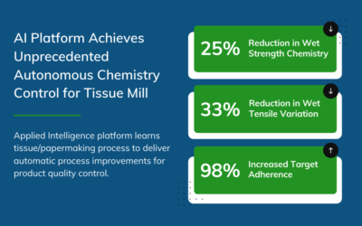
Results
The results are a manufacturing game-changer. Autonomous manufacturing using AI with machine learning allows for improved product quality, optimized use of raw materials with reduced water and energy consumption.
Using a closed-loop controller in conjunction with quality parameter predictions, the mill was able to control its strength chemistry autonomously to ensure optimal chemical feed and adhere to target parameters.
As a result of the artificial intelligence platform, the tissue mill achieved unprecedented autonomous chemistry, allowing for:
Besides Wet Strength, Also Reduced Dry Strength Chemistry by 25%
By: Chitta Ranjan, Ph.D., Director of Science, ProcessMiner, Inc.
Here we will learn the details of data preparation for LSTM models, and build an LSTM Autoencoder for rare-event classification.
This post is a continuation of my previous post Extreme Rare Event Classification using Autoencoders. In the previous post, we talked about the challenges in an extremely rare event data with less than 1% positively labeled data. We built an Autoencoder Classifier for such processes using the concepts of Anomaly Detection.
However, the data we have is a time series. But earlier we used a Dense layer Autoencoder that does not use the temporal features in the data. Therefore, in this post, we will improve on our approach by building an LSTM Autoencoder.
Here, we will learn:
data preparation steps for an LSTM model,
building and implementing LSTM autoencoder, and
using LSTM autoencoder for rare-event classification.
Quick recap on LSTM:
LSTM is a type of Recurrent Neural Network (RNN). RNNs, in general, and LSTM, specifically, are used on sequential or time series data.
These models are capable of automatically extracting effect of past events.
LSTM are known for its ability to extract both long- and short- term effects of pasts event.
In the following, we will go directly to developing an LSTM Autoencoder. It is recommended to read Step-by-step understanding LSTM Autoencoder layers to better understand and further improve the network below.
About the data problem in brief, we have real-world data on sheet breaks from a paper manufacturing. Our objective is to predict the break in advance. Please refer to Extreme Rare Event Classification using Autoencoders for the details on the data, problem, and the classification approach.
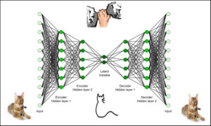
LSTM Autoencoder for Multivariate Data
Figure 1. An LSTM Autoencoder.
In our problem, we have a multivariate time-series data. A multivariate time-series data contains multiple variables observed over a period of time. We will build an LSTM autoencoder on this multivariate time-series to perform rare-event classification. As described in [1], this is achieved by using an anomaly detection approach:
we build an autoencoder on the normal (negatively labeled) data,
use it to reconstruct a new sample,
if the reconstruction error is high, we label it as a sheet-break.
LSTM requires few special data-preprocessing steps. In the following, we will give sufficient attention to these steps.
Let’s get to the implementation.
Libraries
I like to put together the libraries and global constants first.
As mentioned before, LSTM requires a few specific steps in the data preparation. The input to LSTMs are 3-dimensional arrays created from the time-series data. This is an error prone step so we will look at the details.
Read data
The data is taken from [2]. The link to the data is here.
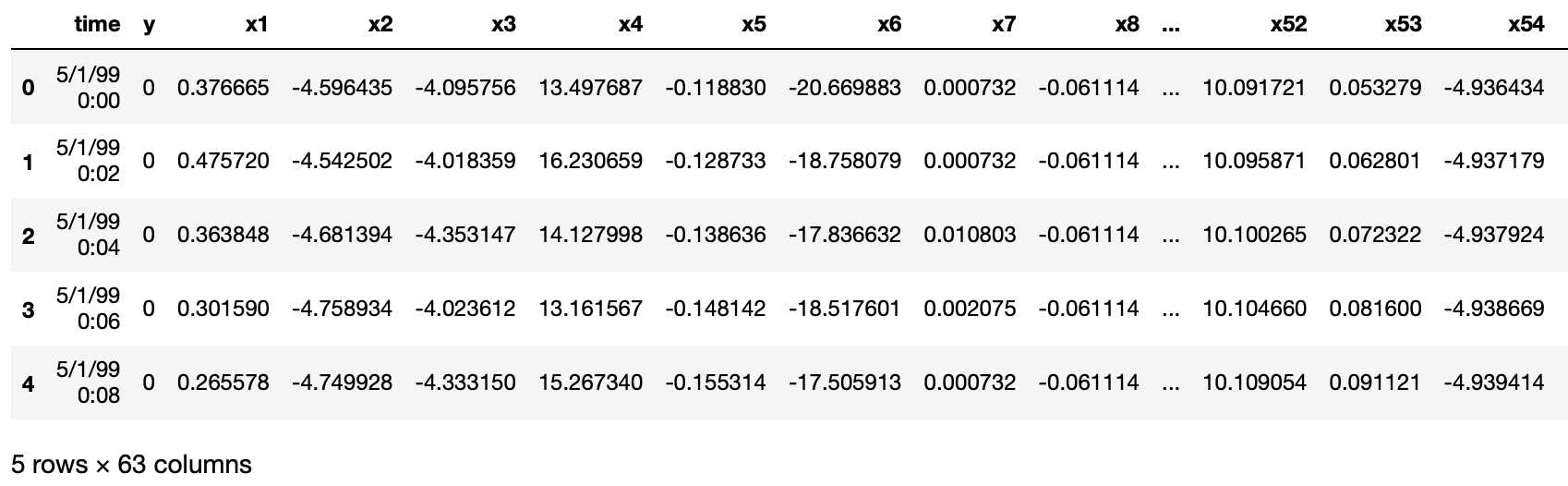
df = pd.read_csv("data/processminer-rare-event-mts - data.csv")
df.head(n=5)  # visualize the data.
Curve Shifting
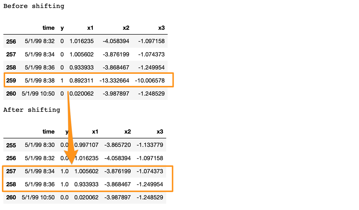
As also mentioned in [1], the objective of this rare-event problem is to predict a sheet-break before it occurs. We will try to predict the break up to 4 minutes in advance. For this data, this is equivalent to shifting the labels up by two rows. It can be done directly with df.y=df.y.shift(-2). However, here we require to do the following,
For any row n with label 1, make (n-2):(n-1) as 1. With this, we are teaching the classifier to predict up to 4 minutes ahead. And,
remove row n. Row n is removed because we are not interested in teaching the classifier to predict a break when it has already happened.
We develop the following function to perform this curve shifting.
sign = lambda x: (1, -1)[x < 0]

def curve_shift(df, shift_by):
    '''
    This function will shift the binary labels in a dataframe.
    The curve shift will be with respect to the 1s.
    For example, if shift is -2, the following process
    will happen: if row n is labeled as 1, then
    - Make row (n+shift_by):(n+shift_by-1) = 1.
    - Remove row n.
    i.e. the labels will be shifted up to 2 rows up.

    Inputs:
    df       A pandas dataframe with a binary labeled column.
             This labeled column should be named as 'y'.
    shift_by An integer denoting the number of rows to shift.

    Output
    df       A dataframe with the binary labels shifted by shift.
    '''

    vector = df['y'].copy()
    for s in range(abs(shift_by)):
        tmp = vector.shift(sign(shift_by))
        tmp = tmp.fillna(0)
        vector += tmp
    labelcol = 'y'
    # Add vector to the df
    df.insert(loc=0, column=labelcol+'tmp', value=vector)
    # Remove the rows with labelcol == 1.
    df = df.drop(df[df[labelcol] == 1].index)
    # Drop labelcol and rename the tmp col as labelcol
    df = df.drop(labelcol, axis=1)
    df = df.rename(columns={labelcol+'tmp': labelcol})
    # Make the labelcol binary
    df.loc[df[labelcol] > 0, labelcol] = 1

    return df
We will now shift our data and verify if the shifting is correct. In the subsequent sections, we have few more test steps. It is recommended to use them to ensure the data preparation steps are working as expected.
print('Before shifting')  # Positive labeled rows before shifting.
one_indexes = df.index[df['y'] == 1]
display(df.iloc[(np.where(np.array(input_y) == 1)[0][0]-5):(np.where(np.array(input_y) == 1)[0][0]+1), ])

# Shift the response column y by 2 rows to do a 4-min ahead prediction.
df = curve_shift(df, shift_by = -2)

print('After shifting')  # Validating if the shift happened correctly.
display(df.iloc[(one_indexes[0]-4):(one_indexes[0]+1), 0:5].head(n=5))
If we note here, we moved the positive label at 5/1/99 8:38 to n-1 and n-2 timestamps, and dropped row n. Also, there is a time difference of more than 2 minutes between a break row and the next row. This is because, when a break occurs, the machine stays in the break status for a while. During this time, we have y = 1 for consecutive rows. In the provided data, these consecutive break rows are deleted to prevent the classifier from learning to predict a break after it has already happened. Refer [2] for details.
Before moving forward, we clean up the data by dropping the time, and two other categorical columns.
# Remove time column, and the categorical columns
df = df.drop(['time', 'x28', 'x61'], axis=1)
Prepare Input Data for LSTM
LSTM is a bit more demanding than other models. Significant amount of time and attention may go in preparing the data that fits an LSTM. However, it is generally worth the effort.
The input data to an LSTM model is a 3-dimensional array. The shape of the array is samples x lookback x features. Let’s understand them,
samples: This is simply the number of observations, or in other words, the number of data points.
lookback: LSTM models are meant to look at the past. Meaning, at time t the LSTM will process data up to (t–lookback) to make a prediction.
features: It is the number of features present in the input data.
First, we will extract the features and response.
input_X = df.loc[:, df.columns != 'y'].values  # converts the df to a numpy array
input_y = df['y'].values

n_features = input_X.shape[1]  # number of features
The input_X here is a 2-dimensional array of size samples x features. We want to be able to transform such a 2D array into a 3D array of size: samples x lookback x features. Refer to Figure 1 above for a visual understanding.
For that, we develop a function temporalize .
def temporalize(X, y, lookback):
    '''
    Inputs
    X         A 2D numpy array ordered by time of shape:
              (n_observations x n_features)
    y         A 1D numpy array with indexes aligned with
              X, i.e. y[i] should correspond to X[i].
              Shape: n_observations.
    lookback  The window size to look back in the past
              records. Shape: a scalar.

    Output
    output_X  A 3D numpy array of shape:
              ((n_observations-lookback-1) x lookback x
              n_features)
    output_y  A 1D array of shape:
              (n_observations-lookback-1), aligned with X.
    '''
    output_X = []
    output_y = []
    for i in range(len(X) - lookback - 1):
        t = []
        for j in range(1, lookback + 1):
            # Gather the past records upto the lookback period
            t.append(X[[(i + j + 1)], :])
        output_X.append(t)
        output_y.append(y[i + lookback + 1])
    return np.squeeze(np.array(output_X)), np.array(output_y)
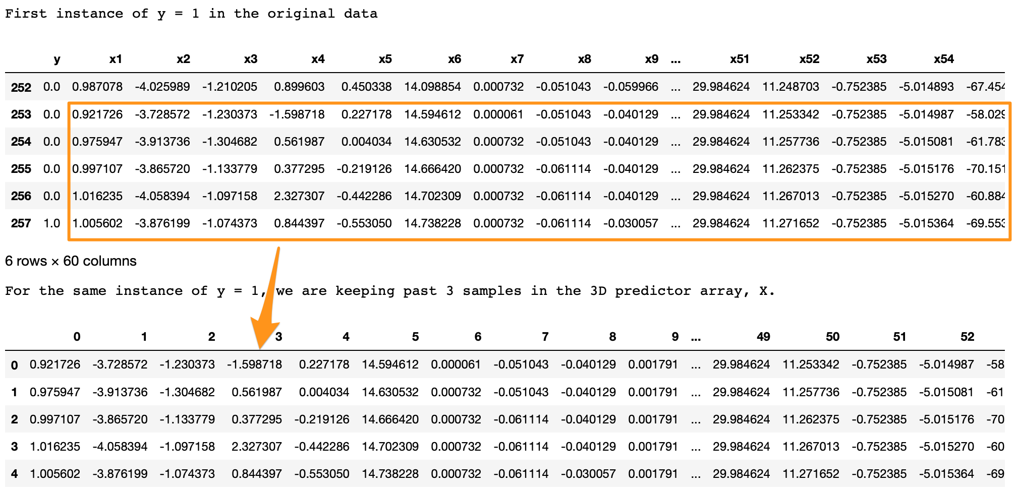
To test and demonstrate this function, we will look at an example below with lookback = 5 .
print('First instance of y = 1 in the original data')
display(df.iloc[(np.where(np.array(input_y) == 1)[0][0]-5):(np.where(np.array(input_y) == 1)[0][0]+1), ])lookback = 5  # Equivalent to 10 min of past data.
# Temporalize the data
X, y = temporalize(X = input_X, y = input_y, lookback = lookback)print('For the same instance of y = 1, we are keeping past 5 samples in the 3D predictor array, X.')
display(pd.DataFrame(np.concatenate(X[np.where(np.array(y) == 1)[0][0]], axis=0 )))
What we are looking for here is,
In the original data, y = 1 at row 257.
With lookback = 5 we want the LSTM to look at the 5 rows before row 257 (including itself).
In the 3D array, X, each 2D block at X[i,:,:] denotes the prediction data that corresponds to y[i] . To draw an analogy, in regression y[i] corresponds to a 1D vector X[i,:] ; in LSTM y[i] corresponds to a 2D array X[i,:,:] .
This 2D block X[i,:,:] should have the predictors at input_X[i,:] and the previous rows up to the given lookback .
As we can see in the output above, the X[i,:,:] block in the bottom is the same as the five past rows of y=1 shown on the top.
Similarly, this is applied for the entire data, for all y’s. The example here is shown for an instance of y=1 for easier visualization.
Split into train, valid, and test
This is straightforward with the sklearn function.
For training the autoencoder, we will be using the X coming from only the negatively labeled data. Therefore, we separate the X corresponding to y = 0.
It is usually better to use a standardized data (transformed to Gaussian with mean 0 and standard deviation 1) for autoencoders.
One common standardization mistake is: we normalize the entire data and then split into train-test. This is incorrect. Test data should be completely unseen to anything during the modeling. We should, therefore, normalize the training data, and use its summary statistics to normalize the test data (for normalization, these statistics are the mean and variances of each feature).
Standardizing this data is a bit tricky. This is because the X matrices are 3D, and we want the standardization to happen with respect to the original 2D data.
To do this, we will require two UDFs.
flatten : This function will re-create the original 2D array from which the 3D arrays were created. This function is the inverse of temporalize, meaning X = flatten(temporalize(X)).
scale : This function will scale a 3D array that we created as inputs to the LSTM.
def flatten(X):
''' Flatten a 3D array. Input X A 3D array for lstm, where the array is sample x timesteps x features. Output flattened_X A 2D array, sample x features. '''
flattened_X = np.empty((X.shape[0], X.shape[2])) # sample x features array.for i in range(X.shape[0]):
flattened_X[i] = X[i, (X.shape[1]-1), :]
return(flattened_X)
def scale(X, scaler):
''' Scale 3D array. Inputs X A 3D array for lstm, where the array is sample x timesteps x features. scaler A scaler object, e.g., sklearn.preprocessing.StandardScaler, sklearn.preprocessing.normalize Output X Scaled 3D array. '''for i in range(X.shape[0]):
X[i, :, :] = scaler.transform(X[i, :, :])
return X
Why didn’t we first normalize the original 2D data and then create the 3D arrays? Because, to do this we will: split the data into train and test, followed by their normalization. However, when we create the 3D arrays on the test data, we lose the initial rows of samples up till the lookback. Splitting into train-valid-test will cause this for both the validation and test sets.
We will fit a Standardization object from sklearn. This function standardizes the data to Normal(0, 1). Note that we require to flatten the X_train_y0 array to pass to the fit function.
# Initialize a scaler using the training data.
scaler = StandardScaler().fit(flatten(X_train_y0))
We will use our UDF, scale, to standardize X_train_y0 with the fitted transform object scaler.
X_train_y0_scaled = scale(X_train_y0, scaler)
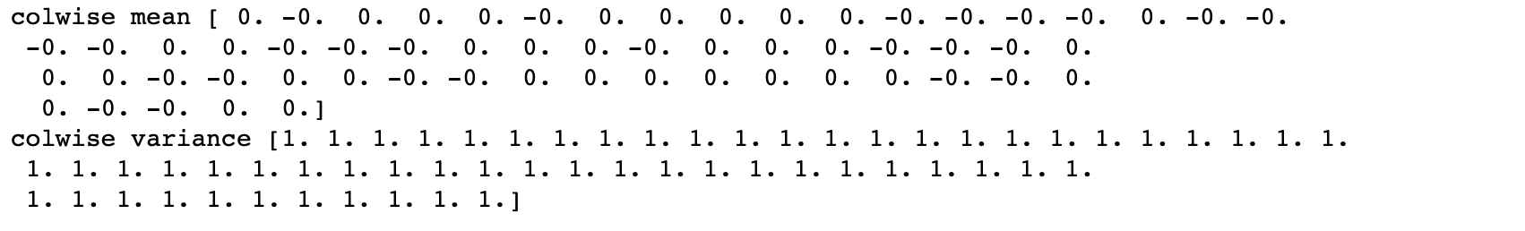
Make sure the scale worked correctly?
A correct transformation of X_train will ensure that the means and variances of each column of the flattened X_train are 0 and 1, respectively. We test this.
All the means and variances outputted above are 0 and 1, respectively. Therefore, the scaling is correct. We will now scale the validation and test sets. We will again use the scaler object on these sets.
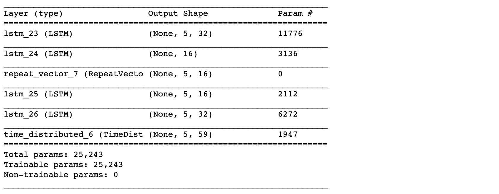
From the summary(), the total number of parameters are 5,331. This is about half of the training size. Hence, this is an appropriate model to fit. To have a bigger architecture, we will need to add regularization, e.g. Dropout, which will be covered in the next post.
Similar to the previous post [1], here we show how we can use an Autoencoder reconstruction error for the rare-event classification. We follow this concept: the autoencoder is expected to reconstruct a noif the reconstruction error is high, we will classify it as a sheet-break.
We will need to determine the threshold for this. Also, note that here we will be using the entire validation set containing both y = 0 or 1.
Note that we have to flatten the arrays to compute the mse.
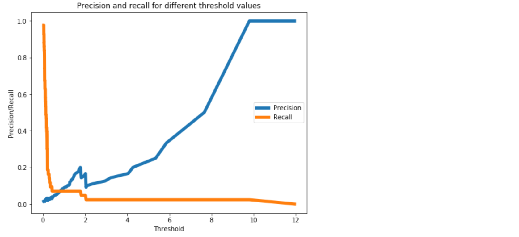
Figure 3. A threshold of 0.3 should provide a reasonable trade-off between precision and recall, as we want to higher recall.
Now, we will perform classification on the test data.
We should not estimate the classification threshold from the test data. It will result in overfitting.
test_x_predictions = lstm_autoencoder.predict(X_test_scaled)
mse = np.mean(np.power(flatten(X_test_scaled) - flatten(test_x_predictions), 2), axis=1)

error_df = pd.DataFrame({'Reconstruction_error': mse,
                        'True_class': y_test.tolist()})

threshold_fixed = 0.3
groups = error_df.groupby('True_class')
fig, ax = plt.subplots()

for name, group in groups:
    ax.plot(group.index, group.Reconstruction_error, marker='o', ms=3.5, linestyle='',
            label= "Break" if name == 1 else "Normal")
ax.hlines(threshold_fixed, ax.get_xlim()[0], ax.get_xlim()[1], colors="r", zorder=100, label='Threshold')
ax.legend()
plt.title("Reconstruction error for different classes")
plt.ylabel("Reconstruction error")
plt.xlabel("Data point index")
plt.show();
Figure 4. Using threshold = 0.8 for classification. The orange and blue dots above the threshold line represents the True Positive and False Positive, respectively.
In Figure 4, the orange and blue dot above the threshold line represents the True Positive and False Positive, respectively. As we can see, we have good number of false positives.
Let’s see the accuracy results.
Test Accuracy
Confusion Matrix
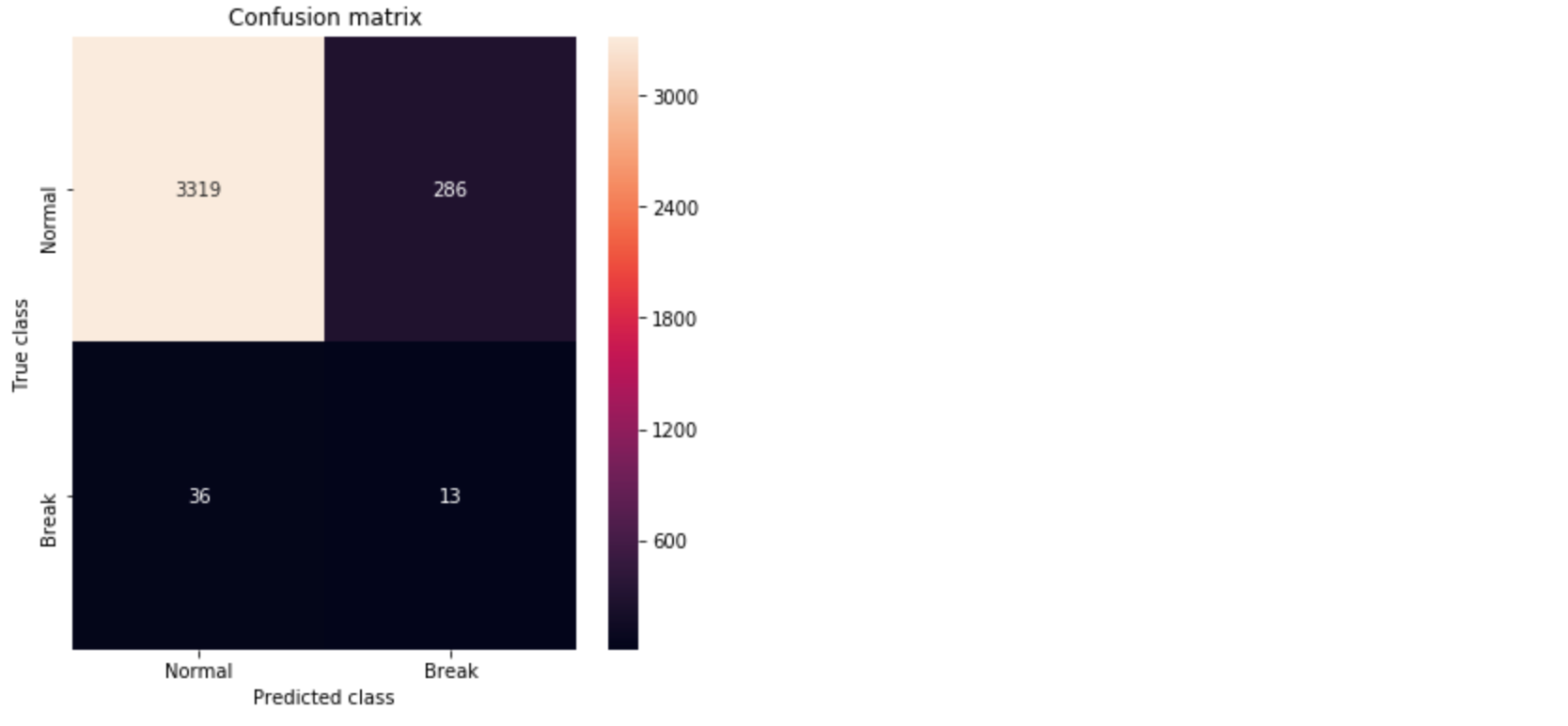
pred_y = [1 if e > threshold_fixed else 0 for e in error_df.Reconstruction_error.values]conf_matrix = confusion_matrix(error_df.True_class, pred_y)

plt.figure(figsize=(6, 6))
sns.heatmap(conf_matrix, xticklabels=LABELS, yticklabels=LABELS, annot=True, fmt="d");
plt.title("Confusion matrix")
plt.ylabel('True class')
plt.xlabel('Predicted class')
plt.show()
Figure 5. Confusion matrix showing the True Positives and False Positives.
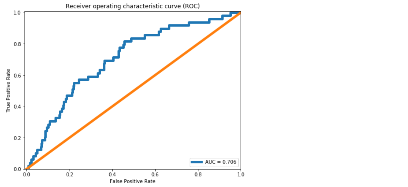
We see approximately 10% improvement in the AUC compared to the dense layer Autoencoder in [1]. From the Confusion Matrix in Figure 5, we could predict 10 out of 39 break instances. As also discussed in [1], this is significant for a paper mill. However, the improvement we achieved in comparison to the dense layer Autoencoder is minor.
The primary reason is LSTM model has more parameters to estimate. It becomes important to use regularization with LSTMs. Regularization and other model improvements will be discussed in the next post.
An LSTM Autoencoder for rare event classification. Contribute to cran2367/lstm_autoencoder_classifier development by…
github.com
What can be done better?
In the next article, we will learn tuning an Autoencoder. We will go over,
CNN LSTM Autoencoder,
Dropout layer,
LSTM Dropout (Dropout_U and Dropout_W)
Gaussian-dropout layer
SELU activation, and
alpha-dropout with SELU activation.
Conclusion
This post continued the work on extreme rare event binary labeled data in [1]. To utilize the temporal patterns, LSTM Autoencoders is used to build a rare event classifier for a multivariate time-series process. Details about the data preprocessing steps for LSTM model are discussed. A simple LSTM Autoencoder model is trained and used for classification. Some improvement in the accuracy over a Dense Autoencoder is found. For further improvement, we will look at ways to improve an Autoencoder with Dropout and other techniques in the next post.
By:Chitta Ranjan, Ph.D., Director of Science, ProcessMiner, Inc.
In this case study, we will learn how to implement an autoencoder for building a rare-event classifier. We will use a real-world rare event dataset.
Background: What is an extreme rare event?
In a rare-event problem, we have an unbalanced dataset. Meaning, we have fewer positively labeled samples than negative. In a typical rare-event problem, the positively labeled data are around 5–10% of the total. In an extremely rare event problem, we have less than 1% positively labeled data. For example, in the dataset used here, it is around 0.6%.
Such extreme rare event problems are quite common in the real-world, for example, sheet-breaks and machine failure in manufacturing, clicks, or purchase in the online industry.
Classifying these rare events is quite challenging. Recently, Deep Learning has been quite extensively used for classification. However, the small number of positively labeled samples prohibits Deep Learning applications. No matter how large the data, the use of Deep Learning gets limited by the amount of positively labeled samples.
Why should we still bother to use Deep Learning?
This is a legitimate question. Why should we not think of using some another Machine Learning approach?
The answer is subjective. We can always go with a Machine Learning approach. To make it work, we can undersample from negatively labeled data to have a close to a balanced dataset. Since we have about 0.6% positively labeled data, the undersampling will result in rougly a dataset that is about 1% of the size of the original data. A Machine Learning approach, e.g. SVM or Random Forest, will still work on a dataset of this size. However, it will have limitations in its accuracy. And we will not utilize the information present in the remaining ~99% of the data.
If the data is sufficient, Deep Learning methods are potentially more capable. It also allows flexibility for model improvement by using different architectures. We will, therefore, attempt to use Deep Learning methods.
In this post, we will learn how we can use a simple dense layers autoencoder to build a rare event classifier. The purpose of this post is to demonstrate the implementation of an Autoencoder for extreme rare-event classification. We will leave the exploration of different architecture and configuration of the Autoencoder on the user. Please share in the comments if you find anything interesting.
Autoencoder for Classification
The autoencoder approach for classification is similar to anomaly detection. In anomaly detection, we learn the pattern of a normal process. Anything that does not follow this pattern is classified as an anomaly. For a binary classification of rare events, we can use a similar approach using autoencoders (derived from here [2]).
Quick revision: What is an autoencoder?
An autoencoder is made of two modules: encoder and decoder
The encoder learns the underlying features of a process; these features are typically in a reduced dimension
The decoder can recreate the original data from these underlying features
How to use an Autoencoder rare-event classification?
We will divide the data into two parts: positively labeled and negatively labeled
The negatively labeled data is treated as a normal state of the process; A normal state is when the process is relentless
We will ignore the positively labeled data, and train an Autoencoder on only negatively labeled data
This Autoencoder has now learned the features of the normal process
A well-trained Autoencoder will predict any new data that is coming from the normal state of the process (as it will have the same pattern or distribution)
Therefore, the reconstruction error will be small
However, if we try to reconstruct data from a rare-event, the Autoencoder will struggle
This will make the reconstruction error high during the rare-event
We can catch such high reconstruction errors and label them as a rare-event prediction
This procedure is similar to anomaly detection methods
Implementation: Data and Problem
This is a binary labeled data from a pulp-and-paper mill for sheet breaks. Sheet breaks is a severe problem in paper manufacturing. A single sheet break causes a loss of several thousand dollars, and the mills see at least one or more breaks every day. This causes millions of dollars of yearly losses and work hazards.
Detecting a break event is challenging due to the nature of the process. As mentioned in [1], even a 5% reduction in the breaks will bring significant benefit to the mills.
The data we have contains about 18k rows collected over 15 days. The column contains the binary labels, with 1 denoting a sheet break. The rest columns are predictors. There are about 124 positive labeled samples (~0.6%).
%matplotlib inline
import matplotlib.pyplot as plt
import seaborn as snsimport pandas as pd
import numpy as np
from pylab import rcParamsimport tensorflow as tf
from keras.models import Model, load_model
from keras.layers import Input, Dense
from keras.callbacks import ModelCheckpoint, TensorBoard
from keras import regularizersfrom sklearn.preprocessing import StandardScaler
from sklearn.model_selection import train_test_split
from sklearn.metrics import confusion_matrix, precision_recall_curve
from sklearn.metrics import recall_score, classification_report, auc, roc_curve
from sklearn.metrics import precision_recall_fscore_support, f1_scorefrom numpy.random import seed
seed(1)
from tensorflow import set_random_seed
set_random_seed(2)SEED = 123 #used to help randomly select the data points
DATA_SPLIT_PCT = 0.2rcParams['figure.figsize'] = 8, 6
LABELS = ["Normal","Break"]
Note that we are setting the random seeds for the reproducibility of the result.
Data Preprocessing
Now, we read and prepare the data.[/vc_column_text][vc_column_text]
The objective of this rare-event problem is to predict a sheet-break before it occurs. We will try to predict the break 4 minutes in advance. To build this model, we will shift the labels 2 rows up (which corresponds to 4 minutes). We can do this as:However, in this problem, we would want to do the shifting as: if row n is positively labeled:
make rows (n-2) and (n-1) equal to 1 | This will help the classifier learn up to 4 minutes ahead prediction
Delete row n, bsecause we do not want the classifier to learn to predict a break when it has happened
We will develop the following UDF for this curve shifting.[/vc_column_text][vc_column_text]
sign = lambda x: (1, -1)[x < 0]

def curve_shift(df, shift_by):
    '''
    This function will shift the binary labels in a dataframe.
    The curve shift will be with respect to the 1s.
    For example, if shift is -2, the following process
    will happen: if row n is labeled as 1, then
    - Make row (n+shift_by):(n+shift_by-1) = 1.
    - Remove row n.
    i.e. the labels will be shifted up to 2 rows up.

    Inputs:
    df       A pandas dataframe with a binary labeled column.
             This labeled column should be named as 'y'.
    shift_by An integer denoting the number of rows to shift.

    Output
    df       A dataframe with the binary labels shifted by shift.
    '''

    vector = df['y'].copy()
    for s in range(abs(shift_by)):
        tmp = vector.shift(sign(shift_by))
        tmp = tmp.fillna(0)
        vector += tmp
    labelcol = 'y'
    # Add vector to the df
    df.insert(loc=0, column=labelcol+'tmp', value=vector)
    # Remove the rows with labelcol == 1.
    df = df.drop(df[df[labelcol] == 1].index)
    # Drop labelcol and rename the tmp col as labelcol
    df = df.drop(labelcol, axis=1)
    df = df.rename(columns={labelcol+'tmp': labelcol})
    # Make the labelcol binary
    df.loc[df[labelcol] > 0, labelcol] = 1

    return df
Before moving forward, we will drop the time, and also the categorical columns for simplicity.
# Remove time column, and the categorical columns
df = df.drop(['time', 'x28', 'x61'], axis=1)
Now, we divide the data into train, valid, and test sets. Then we will take the subset of data with only 0s to train the autoencoder.
Initialization: First, we will initialize Autoencoder architecture. We are building a simple autoencoder. More complex architectures and other configurations should be explored.
We should not estimate the classification threshold from the test data. It will result in overfitting.
test_x_predictions = autoencoder.predict(df_test_x_rescaled)
mse = np.mean(np.power(df_test_x_rescaled - test_x_predictions, 2), axis=1)
error_df_test = pd.DataFrame({'Reconstruction_error': mse,
                        'True_class': df_test['y']})
error_df_test = error_df_test.reset_index()threshold_fixed = 0.4
groups = error_df_test.groupby('True_class')fig, ax = plt.subplots()for name, group in groups:
    ax.plot(group.index, group.Reconstruction_error, marker='o', ms=3.5, linestyle='',
            label= "Break" if name == 1 else "Normal")
ax.hlines(threshold_fixed, ax.get_xlim()[0], ax.get_xlim()[1], colors="r", zorder=100, label='Threshold')
ax.legend()
plt.title("Reconstruction error for different classes")
plt.ylabel("Reconstruction error")
plt.xlabel("Data point index")
plt.show();
pred_y = [1 if e > threshold_fixed else 0 for e in error_df.Reconstruction_error.values]conf_matrix = confusion_matrix(error_df.True_class, pred_y)plt.figure(figsize=(12, 12))
sns.heatmap(conf_matrix, xticklabels=LABELS, yticklabels=LABELS, annot=True, fmt="d");
plt.title("Confusion matrix")
plt.ylabel('True class')
plt.xlabel('Predicted class')
plt.show()
We could predict 8 out of 41 breaks instances. Note that these instances include 2 or 4 minute ahead predictions. This is around 20%, which is a good recall rate for the paper industry. The False Positive Rate is around 6%. This is not ideal but not terrible for a mill.
Still, this model can be further improved to increase the recall rate with smaller False Positive Rate. We will look at the AUC below and then talk about the next approach for improvement.
cran2367/autoencoder_classifier Autoencoder model for rare event classification. Contribute to cran2367/autoencoder_classifier development by creating… github.com What Can Be Done Better Here? Autoencoder Optimization Autoencoders are a nonlinear extension of PCA. However, the conventional Autoencoder developed above does not follow the principles of PCA. In Build the right Autoencoder — Tune and Optimize using PCA principles. Part I and Part II, the required PCA principles that should be incorporated in an Autoencoder for optimization are explained and implemented.
LSTM Autoencoder The problem discussed here is a (multivariate) time series. However, in the Autoencoder model, we are not taking into account the temporal information/patterns. In the next post, we will explore if it is possible with an RNN. We will try an LSTM autoencoder.
Conclusion
We worked on an extreme rare event binary labeled data from a paper mill to build an Autoencoder Classifier. We achieved reasonable accuracy. The purpose here was to demonstrate the use of a basic Autoencoder for rare event classification. We will further work on developing other methods, including an LSTM Autoencoder that can extract the temporal features for better accuracy.
In this post, we will learn about using a nonlinear correlation estimation function in R. We will also look at a few examples.
Background
Correlation estimations are commonly used in various data mining applications. In my experience, nonlinear correlations are quite common in various processes. Due to this, nonlinear models, such as SVM, are employed for regression, classification, etc. However, there are not many approaches to estimate nonlinear correlations between two variables.
Typically linear correlations are estimated. However, the data may have a nonlinear correlation but little to no linear correlation. In such cases, nonlinearly correlated variables are sometimes overlooked during data exploration or variable selection in high-dimensional data.
We have developed a new nonlinear correlation estimator:
nlcor
This estimator comes useful in data exploration and also variable selection for nonlinear predictive models, such as SVM.
Installing
To install
nlcor
in R, follow these steps:
Install the devtools package. You can do this from CRAN. You can do it directly in R console by typing,
> install.packages("devtools")
2. Load the devtools package.
> library(devtools)
3. Install
nlcor
from its GitHub repository by typing this in R console.
> install_github("ProcessMiner/nlcor")
Nonlinear Correlation Estimator: Nlcor
In this package, we provide an implementation of a nonlinear correlation estimation method using an adaptive local linear correlation computation in
nlcor
The function
nlcor
returns the nonlinear correlation estimate, the corresponding adjusted p-value, and an optional plot visualizing the nonlinear relationships.
The correlation estimate will be between 0 and 1. The higher the value the more is the nonlinear correlation. Unlike linear correlations, a negative value is not valid here. Due to multiple local correlation computations, the net p-value of the correlation estimate is adjusted (to avoid false positives). The plot visualizes the local linear correlations.
In the following, we will show its usage with a few examples. In the given examples, the linear correlations between
x
and
nlcor
is small, however, there is a visible nonlinear correlation between them. This package contains the data for these examples and can be used for testing the package.
nlcor
package has few sample
x
and
y
vectors that are demonstrated in the following examples.
First, we will load the package.
> library(nlcor)
Example 1. A data with cyclic nonlinear correlation.
> plot(x1, y1)
The linear correlation of the data is,
> cor(x1, y1)
[1] 0.008001837
As expected, the correlation is close to zero. We estimate the nonlinear correlation using
The plot shows the piecewise linear correlations present in the data.
Example 2. A data with non-uniform piecewise linear correlations.
> plot(x2, y2)
The linear correlation of the data is,
> cor(x2, y2)
[1] 0.828596
The linear correlation is quite high in this data. However, there is significant and higher nonlinear correlation present in the data. This data emulates the scenario where the correlation changes its direction after a point. Sometimes that change point is in the middle causing the linear correlation to be close to zero. Here we show an example when the change point is off-center to show that the implementation works in non-uniform cases.
could estimate the piecewise correlations in a non-uniform scenario. Also, the nonlinear correlation comes out to be higher than the linear correlation.
Example 3. A data with higher and multiple frequency variations.
> plot(x3, y3)
The linear correlation of the data is,
> cor(x3, y3)
[1] -0.1337304
The linear correlation is expectedly small, albeit not close to zero due to some linearity.
Here we show we can refine the granularity of the correlation computation.
could identify the granular piecewise correlations. In this data, the p-value still remains extremely small—the correlation is statistically significant.
Summary
This package provides an implementation of an efficient heuristic to compute the nonlinear correlations between numeric vectors. The heuristic works by adaptively identifying multiple local regions of linear correlations to estimate the overall nonlinear correlation. Its usages are demonstrated here with few examples.
The goal of this project was to autonomously control part of a tissue mill’s continuous manufacturing process using artificial intelligence and predictive analytics to reduce raw material consumption while maintaining the product quality with specification limit.
Here we will learn the details of data preparation for LSTM models, and build an LSTM Autoencoder for rare-event classification. This post is a continuation of my previous post-Extreme Rare Event Classification using Autoencoders. In the previous post, we talked about the challenges in an extremely rare event data with less than 1% positively labeled data.
We use cookies to optimize our website and our service.
Functional
Always active
The technical storage or access is strictly necessary for the legitimate purpose of enabling the use of a specific service explicitly requested by the subscriber or user, or for the sole purpose of carrying out the transmission of a communication over an electronic communications network.
Preferences
The technical storage or access is necessary for the legitimate purpose of storing preferences that are not requested by the subscriber or user.
Statistics
The technical storage or access that is used exclusively for statistical purposes.The technical storage or access that is used exclusively for anonymous statistical purposes. Without a subpoena, voluntary compliance on the part of your Internet Service Provider, or additional records from a third party, information stored or retrieved for this purpose alone cannot usually be used to identify you.
Marketing
The technical storage or access is required to create user profiles to send advertising, or to track the user on a website or across several websites for similar marketing purposes.
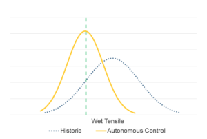
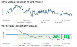
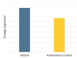
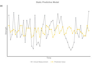
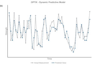
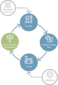
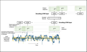 Figure 1. An LSTM Autoencoder.