
By: Chitta Ranjan, Ph.D., Director of Science, ProcessMiner, Inc.
Here we will learn the details of data preparation for LSTM models, and build an LSTM Autoencoder for rare-event classification.
This post is a continuation of my previous post Extreme Rare Event Classification using Autoencoders. In the previous post, we talked about the challenges in an extremely rare event data with less than 1% positively labeled data. We built an Autoencoder Classifier for such processes using the concepts of Anomaly Detection.
However, the data we have is a time series. But earlier we used a Dense layer Autoencoder that does not use the temporal features in the data. Therefore, in this post, we will improve on our approach by building an LSTM Autoencoder.
Here, we will learn:
- data preparation steps for an LSTM model,
- building and implementing LSTM autoencoder, and
- using LSTM autoencoder for rare-event classification.
Quick recap on LSTM:
- LSTM is a type of Recurrent Neural Network (RNN). RNNs, in general, and LSTM, specifically, are used on sequential or time series data.
- These models are capable of automatically extracting effect of past events.
- LSTM are known for its ability to extract both long- and short- term effects of pasts event.
In the following, we will go directly to developing an LSTM Autoencoder. It is recommended to read Step-by-step understanding LSTM Autoencoder layers to better understand and further improve the network below.
About the data problem in brief, we have real-world data on sheet breaks from a paper manufacturing. Our objective is to predict the break in advance. Please refer to Extreme Rare Event Classification using Autoencoders for the details on the data, problem, and the classification approach.
LSTM Autoencoder for Multivariate Data
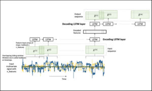 Figure 1. An LSTM Autoencoder.
In our problem, we have a multivariate time-series data. A multivariate time-series data contains multiple variables observed over a period of time. We will build an LSTM autoencoder on this multivariate time-series to perform rare-event classification. As described in [1], this is achieved by using an anomaly detection approach:
- we build an autoencoder on the normal (negatively labeled) data,
- use it to reconstruct a new sample,
- if the reconstruction error is high, we label it as a sheet-break.
LSTM requires few special data-preprocessing steps. In the following, we will give sufficient attention to these steps.
Let’s get to the implementation.
Libraries
I like to put together the libraries and global constants first.
%matplotlib inline
import matplotlib.pyplot as plt
import seaborn as sns

import pandas as pd
import numpy as np
from pylab import rcParams

import tensorflow as tf
from keras import optimizers, Sequential
from keras.models import Model
from keras.utils import plot_model
from keras.layers import Dense, LSTM, RepeatVector, TimeDistributed
from keras.callbacks import ModelCheckpoint, TensorBoard

from sklearn.preprocessing import StandardScaler
from sklearn.model_selection import train_test_split
from sklearn.metrics import confusion_matrix, precision_recall_curve
from sklearn.metrics import recall_score, classification_report, auc, roc_curve
from sklearn.metrics import precision_recall_fscore_support, f1_score

from numpy.random import seed
seed(7)
from tensorflow import set_random_seed
set_random_seed(11)from sklearn.model_selection import train_test_split

SEED = 123 #used to help randomly select the data points
DATA_SPLIT_PCT = 0.2

rcParams['figure.figsize'] = 8, 6
LABELS = ["Normal","Break"]
Data Preparation
As mentioned before, LSTM requires a few specific steps in the data preparation. The input to LSTMs are 3-dimensional arrays created from the time-series data. This is an error prone step so we will look at the details.
Read data
The data is taken from [2]. The link to the data is here.
df = pd.read_csv("data/processminer-rare-event-mts - data.csv")
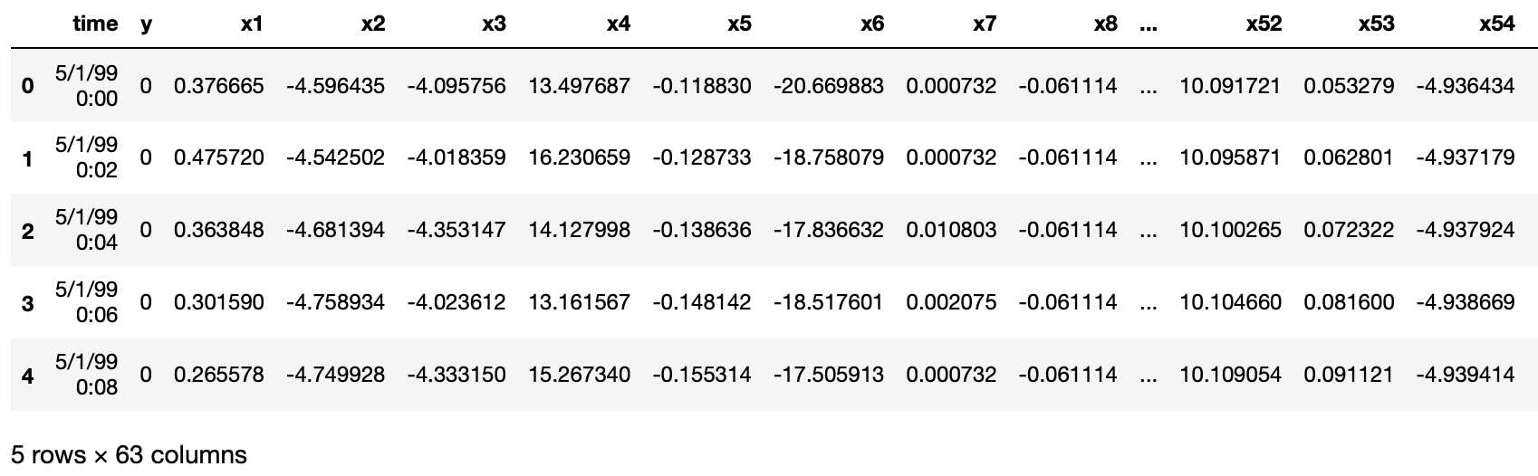
df.head(n=5) # visualize the data.

Curve Shifting
As also mentioned in [1], the objective of this rare-event problem is to predict a sheet-break before it occurs. We will try to predict the break up to 4 minutes in advance. For this data, this is equivalent to shifting the labels up by two rows. It can be done directly with df.y=df.y.shift(-2). However, here we require to do the following,
- For any row n with label 1, make (n-2):(n-1) as 1. With this, we are teaching the classifier to predict up to 4 minutes ahead. And,
- remove row n. Row n is removed because we are not interested in teaching the classifier to predict a break when it has already happened.
We develop the following function to perform this curve shifting.
sign = lambda x: (1, -1)[x < 0]

def curve_shift(df, shift_by):
    '''
    This function will shift the binary labels in a dataframe.
    The curve shift will be with respect to the 1s.
    For example, if shift is -2, the following process
    will happen: if row n is labeled as 1, then
    - Make row (n+shift_by):(n+shift_by-1) = 1.
    - Remove row n.
    i.e. the labels will be shifted up to 2 rows up.

    Inputs:
    df       A pandas dataframe with a binary labeled column.
             This labeled column should be named as 'y'.
    shift_by An integer denoting the number of rows to shift.

    Output
    df       A dataframe with the binary labels shifted by shift.
    '''

    vector = df['y'].copy()
    for s in range(abs(shift_by)):
        tmp = vector.shift(sign(shift_by))
        tmp = tmp.fillna(0)
        vector += tmp
    labelcol = 'y'
    # Add vector to the df
    df.insert(loc=0, column=labelcol+'tmp', value=vector)
    # Remove the rows with labelcol == 1.
    df = df.drop(df[df[labelcol] == 1].index)
    # Drop labelcol and rename the tmp col as labelcol
    df = df.drop(labelcol, axis=1)
    df = df.rename(columns={labelcol+'tmp': labelcol})
    # Make the labelcol binary
    df.loc[df[labelcol] > 0, labelcol] = 1

    return df
We will now shift our data and verify if the shifting is correct. In the subsequent sections, we have few more test steps. It is recommended to use them to ensure the data preparation steps are working as expected.
print('Before shifting')  # Positive labeled rows before shifting.
one_indexes = df.index[df['y'] == 1]
display(df.iloc[(np.where(np.array(input_y) == 1)[0][0]-5):(np.where(np.array(input_y) == 1)[0][0]+1), ])

# Shift the response column y by 2 rows to do a 4-min ahead prediction.
df = curve_shift(df, shift_by = -2)

print('After shifting')  # Validating if the shift happened correctly.
display(df.iloc[(one_indexes[0]-4):(one_indexes[0]+1), 0:5].head(n=5))

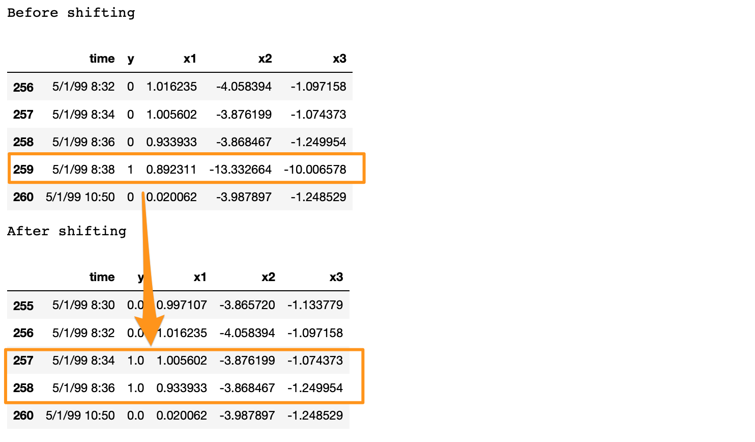
If we note here, we moved the positive label at 5/1/99 8:38 to n-1 and n-2 timestamps, and dropped row n. Also, there is a time difference of more than 2 minutes between a break row and the next row. This is because, when a break occurs, the machine stays in the break status for a while. During this time, we have y = 1 for consecutive rows. In the provided data, these consecutive break rows are deleted to prevent the classifier from learning to predict a break after it has already happened. Refer [2] for details.
Before moving forward, we clean up the data by dropping the time, and two other categorical columns.
# Remove time column, and the categorical columns
df = df.drop(['time', 'x28', 'x61'], axis=1)
Prepare Input Data for LSTM
LSTM is a bit more demanding than other models. Significant amount of time and attention may go in preparing the data that fits an LSTM. However, it is generally worth the effort.
The input data to an LSTM model is a 3-dimensional array. The shape of the array is samples x lookback x features. Let’s understand them,
- samples: This is simply the number of observations, or in other words, the number of data points.
- lookback: LSTM models are meant to look at the past. Meaning, at time t the LSTM will process data up to (t–lookback) to make a prediction.
- features: It is the number of features present in the input data.
First, we will extract the features and response.
input_X = df.loc[:, df.columns != 'y'].values  # converts the df to a numpy array
input_y = df['y'].values

n_features = input_X.shape[1]  # number of features
The input_X here is a 2-dimensional array of size samples x features. We want to be able to transform such a 2D array into a 3D array of size: samples x lookback x features. Refer to Figure 1 above for a visual understanding.
For that, we develop a function temporalize .
def temporalize(X, y, lookback):
    '''
    Inputs
    X         A 2D numpy array ordered by time of shape:
              (n_observations x n_features)
    y         A 1D numpy array with indexes aligned with
              X, i.e. y[i] should correspond to X[i].
              Shape: n_observations.
    lookback  The window size to look back in the past
              records. Shape: a scalar.

    Output
    output_X  A 3D numpy array of shape:
              ((n_observations-lookback-1) x lookback x
              n_features)
    output_y  A 1D array of shape:
              (n_observations-lookback-1), aligned with X.
    '''
    output_X = []
    output_y = []
    for i in range(len(X) - lookback - 1):
        t = []
        for j in range(1, lookback + 1):
            # Gather the past records upto the lookback period
            t.append(X[[(i + j + 1)], :])
        output_X.append(t)
        output_y.append(y[i + lookback + 1])
    return np.squeeze(np.array(output_X)), np.array(output_y)
To test and demonstrate this function, we will look at an example below with lookback = 5 .
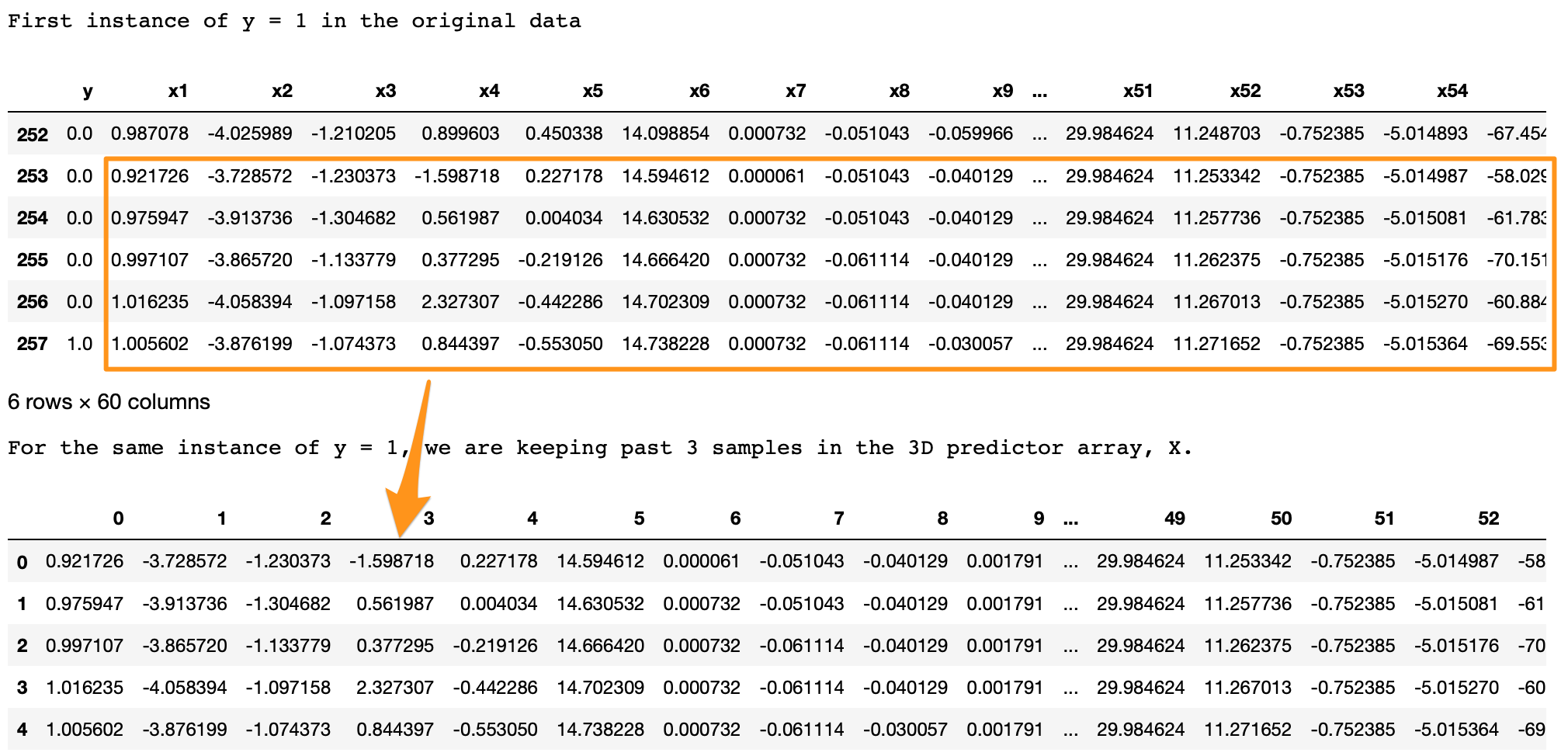
print('First instance of y = 1 in the original data')
display(df.iloc[(np.where(np.array(input_y) == 1)[0][0]-5):(np.where(np.array(input_y) == 1)[0][0]+1), ])lookback = 5  # Equivalent to 10 min of past data.
# Temporalize the data
X, y = temporalize(X = input_X, y = input_y, lookback = lookback)print('For the same instance of y = 1, we are keeping past 5 samples in the 3D predictor array, X.')
display(pd.DataFrame(np.concatenate(X[np.where(np.array(y) == 1)[0][0]], axis=0 )))

What we are looking for here is,
- In the original data, y = 1 at row 257.
- With
lookback = 5we want the LSTM to look at the 5 rows before row 257 (including itself). - In the 3D array,
X, each 2D block atX[i,:,:]denotes the prediction data that corresponds toy[i]. To draw an analogy, in regressiony[i]corresponds to a 1D vectorX[i,:]; in LSTMy[i]corresponds to a 2D arrayX[i,:,:]. - This 2D block
X[i,:,:]should have the predictors atinput_X[i,:]and the previous rows up to the givenlookback. - As we can see in the output above, the
X[i,:,:]block in the bottom is the same as the five past rows of y=1 shown on the top. - Similarly, this is applied for the entire data, for all y’s. The example here is shown for an instance of y=1 for easier visualization.
Split into train, valid, and test
This is straightforward with the sklearn function.
X_train, X_test, y_train, y_test = train_test_split(np.array(X), np.array(y), test_size=DATA_SPLIT_PCT, random_state=SEED)X_train, X_valid, y_train, y_valid = train_test_split(X_train, y_train, test_size=DATA_SPLIT_PCT, random_state=SEED)
For training the autoencoder, we will be using the X coming from only the negatively labeled data. Therefore, we separate the X corresponding to y = 0.
X_train_y0 = X_train[y_train==0]
X_train_y1 = X_train[y_train==1]X_valid_y0 = X_valid[y_valid==0]
X_valid_y1 = X_valid[y_valid==1]
We will reshape the X’s into the required 3D dimension: sample x lookback x features.
X_train = X_train.reshape(X_train.shape[0], lookback, n_features)
X_train_y0 = X_train_y0.reshape(X_train_y0.shape[0], lookback, n_features)
X_train_y1 = X_train_y1.reshape(X_train_y1.shape[0], lookback, n_features)X_valid = X_valid.reshape(X_valid.shape[0], lookback, n_features)
X_valid_y0 = X_valid_y0.reshape(X_valid_y0.shape[0], lookback, n_features)
X_valid_y1 = X_valid_y1.reshape(X_valid_y1.shape[0], lookback, n_features)X_test = X_test.reshape(X_test.shape[0], lookback, n_features)
Standardize the Data
It is usually better to use a standardized data (transformed to Gaussian with mean 0 and standard deviation 1) for autoencoders.
One common standardization mistake is: we normalize the entire data and then split into train-test. This is incorrect. Test data should be completely unseen to anything during the modeling. We should, therefore, normalize the training data, and use its summary statistics to normalize the test data (for normalization, these statistics are the mean and variances of each feature).
Standardizing this data is a bit tricky. This is because the X matrices are 3D, and we want the standardization to happen with respect to the original 2D data.
To do this, we will require two UDFs.
flatten: This function will re-create the original 2D array from which the 3D arrays were created. This function is the inverse oftemporalize, meaningX = flatten(temporalize(X)).scale: This function will scale a 3D array that we created as inputs to the LSTM.
def flatten(X):
    '''
    Flatten a 3D array.

    Input
    X            A 3D array for lstm, where the array is sample x timesteps x features.

    Output
    flattened_X  A 2D array, sample x features.
    '''
    flattened_X = np.empty((X.shape[0], X.shape[2]))  # sample x features array.
    for i in range(X.shape[0]):
        flattened_X[i] = X[i, (X.shape[1]-1), :]
    return(flattened_X)

def scale(X, scaler):
    '''
    Scale 3D array.

    Inputs
    X            A 3D array for lstm, where the array is sample x timesteps x features.
    scaler       A scaler object, e.g., sklearn.preprocessing.StandardScaler, sklearn.preprocessing.normalize

    Output
    X            Scaled 3D array.
    '''
    for i in range(X.shape[0]):
        X[i, :, :] = scaler.transform(X[i, :, :])

    return X
Why didn’t we first normalize the original 2D data and then create the 3D arrays? Because, to do this we will: split the data into train and test, followed by their normalization. However, when we create the 3D arrays on the test data, we lose the initial rows of samples up till the lookback. Splitting into train-valid-test will cause this for both the validation and test sets.
We will fit a Standardization object from sklearn. This function standardizes the data to Normal(0, 1). Note that we require to flatten the X_train_y0 array to pass to the fit function.
# Initialize a scaler using the training data.
scaler = StandardScaler().fit(flatten(X_train_y0))
We will use our UDF, scale, to standardize X_train_y0 with the fitted transform object scaler.
X_train_y0_scaled = scale(X_train_y0, scaler)
Make sure the scale worked correctly?
A correct transformation of X_train will ensure that the means and variances of each column of the flattened X_train are 0 and 1, respectively. We test this.
a = flatten(X_train_y0_scaled)
print('colwise mean', np.mean(a, axis=0).round(6))
print('colwise variance', np.var(a, axis=0))

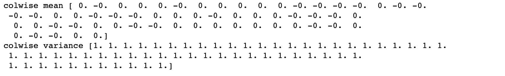
All the means and variances outputted above are 0 and 1, respectively. Therefore, the scaling is correct. We will now scale the validation and test sets. We will again use the scaler object on these sets.
X_valid_scaled = scale(X_valid, scaler)
X_valid_y0_scaled = scale(X_valid_y0, scaler)X_test_scaled = scale(X_test, scaler)
LSTM Autoencoder Training
We will, first, initialize few variables.
timesteps =  X_train_y0_scaled.shape[1] # equal to the lookback
n_features =  X_train_y0_scaled.shape[2] # 59

epochs = 200
batch = 64
lr = 0.0001
We, now, develop a simple architecture.
lstm_autoencoder = Sequential()
# Encoder
lstm_autoencoder.add(LSTM(32, activation='relu', input_shape=(timesteps, n_features), return_sequences=True))
lstm_autoencoder.add(LSTM(16, activation='relu', return_sequences=False))
lstm_autoencoder.add(RepeatVector(timesteps))
# Decoder
lstm_autoencoder.add(LSTM(16, activation='relu', return_sequences=True))
lstm_autoencoder.add(LSTM(32, activation='relu', return_sequences=True))
lstm_autoencoder.add(TimeDistributed(Dense(n_features)))

lstm_autoencoder.summary()

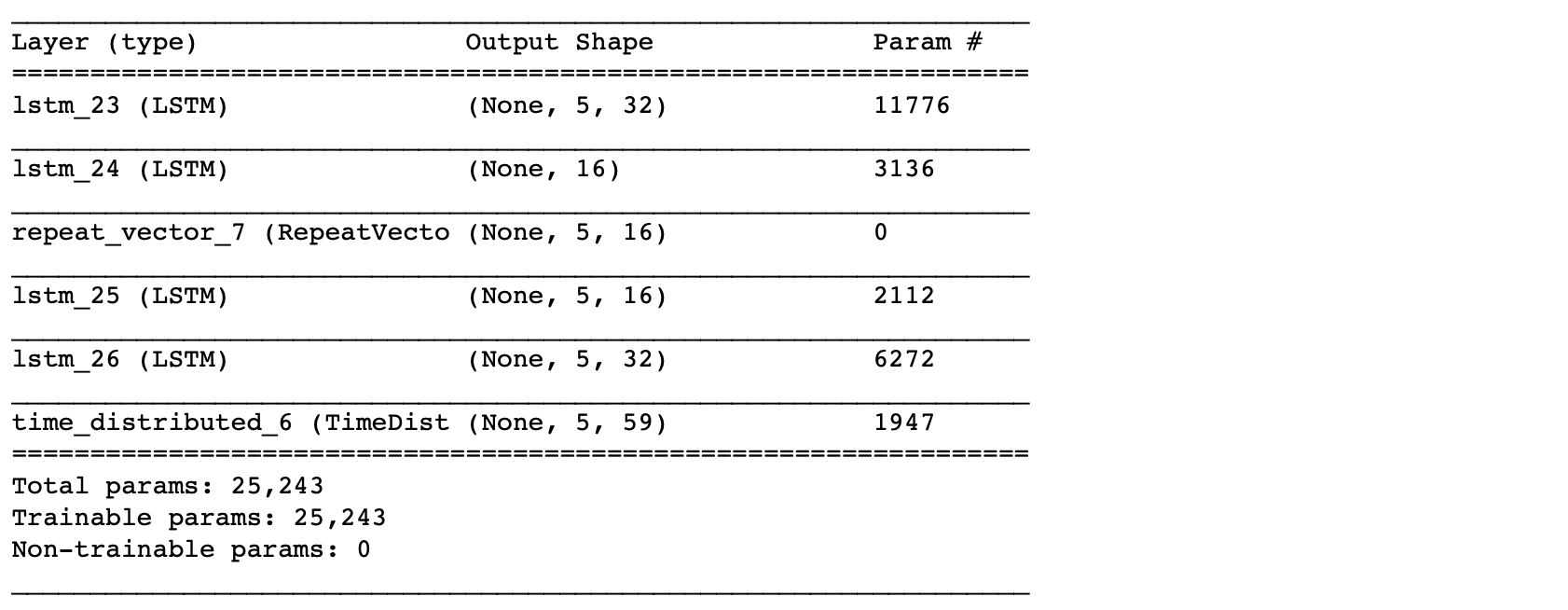
From the summary(), the total number of parameters are 5,331. This is about half of the training size. Hence, this is an appropriate model to fit. To have a bigger architecture, we will need to add regularization, e.g. Dropout, which will be covered in the next post.
Now, we will train the autoencoder.
adam = optimizers.Adam(lr)
lstm_autoencoder.compile(loss='mse', optimizer=adam)

cp = ModelCheckpoint(filepath="lstm_autoencoder_classifier.h5",
                               save_best_only=True,
                               verbose=0)

tb = TensorBoard(log_dir='./logs',
                histogram_freq=0,
                write_graph=True,
                write_images=True)

lstm_autoencoder_history = lstm_autoencoder.fit(X_train_y0_scaled, X_train_y0_scaled,
                                                epochs=epochs,
                                                batch_size=batch,
                                                validation_data=(X_valid_y0_scaled, X_valid_y0_scaled),
                                                verbose=2).history


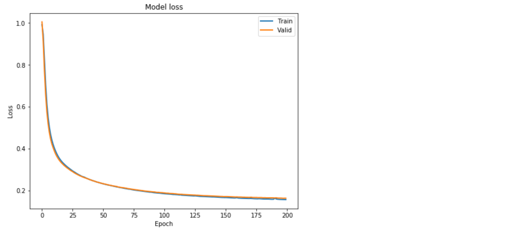
Plotting the change in the loss over the epochs.
plt.plot(lstm_autoencoder_history['loss'], linewidth=2, label='Train')
plt.plot(lstm_autoencoder_history['val_loss'], linewidth=2, label='Valid')
plt.legend(loc='upper right')
plt.title('Model loss')
plt.ylabel('Loss')
plt.xlabel('Epoch')
plt.show()

Classification
Similar to the previous post [1], here we show how we can use an Autoencoder reconstruction error for the rare-event classification. We follow this concept: the autoencoder is expected to reconstruct a noif the reconstruction error is high, we will classify it as a sheet-break.
We will need to determine the threshold for this. Also, note that here we will be using the entire validation set containing both y = 0 or 1.
valid_x_predictions = lstm_autoencoder.predict(X_valid_scaled)
mse = np.mean(np.power(flatten(X_valid_scaled) - flatten(valid_x_predictions), 2), axis=1)
error_df = pd.DataFrame({'Reconstruction_error': mse,
'True_class': y_valid.tolist()})
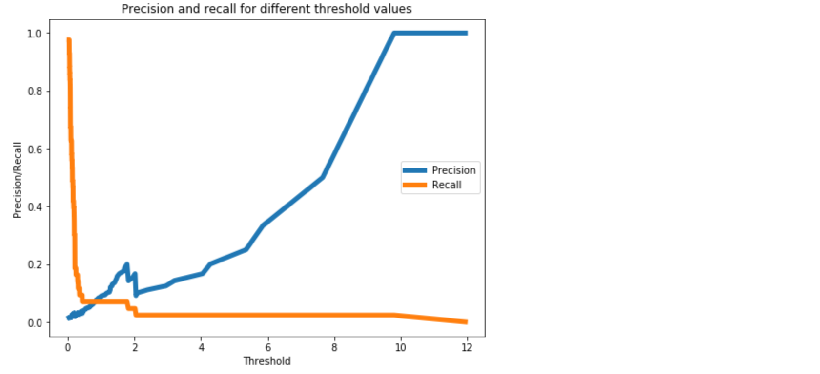
precision_rt, recall_rt, threshold_rt = precision_recall_curve(error_df.True_class, error_df.Reconstruction_error)
plt.plot(threshold_rt, precision_rt[1:], label="Precision",linewidth=5)
plt.plot(threshold_rt, recall_rt[1:], label="Recall",linewidth=5)
plt.title('Precision and recall for different threshold values')
plt.xlabel('Threshold')
plt.ylabel('Precision/Recall')
plt.legend()
plt.show()
Note that we have to flatten the arrays to compute the mse.

Now, we will perform classification on the test data.
We should not estimate the classification threshold from the test data. It will result in overfitting.
test_x_predictions = lstm_autoencoder.predict(X_test_scaled)
mse = np.mean(np.power(flatten(X_test_scaled) - flatten(test_x_predictions), 2), axis=1)

error_df = pd.DataFrame({'Reconstruction_error': mse,
                        'True_class': y_test.tolist()})

threshold_fixed = 0.3
groups = error_df.groupby('True_class')
fig, ax = plt.subplots()

for name, group in groups:
    ax.plot(group.index, group.Reconstruction_error, marker='o', ms=3.5, linestyle='',
            label= "Break" if name == 1 else "Normal")
ax.hlines(threshold_fixed, ax.get_xlim()[0], ax.get_xlim()[1], colors="r", zorder=100, label='Threshold')
ax.legend()
plt.title("Reconstruction error for different classes")
plt.ylabel("Reconstruction error")
plt.xlabel("Data point index")
plt.show();

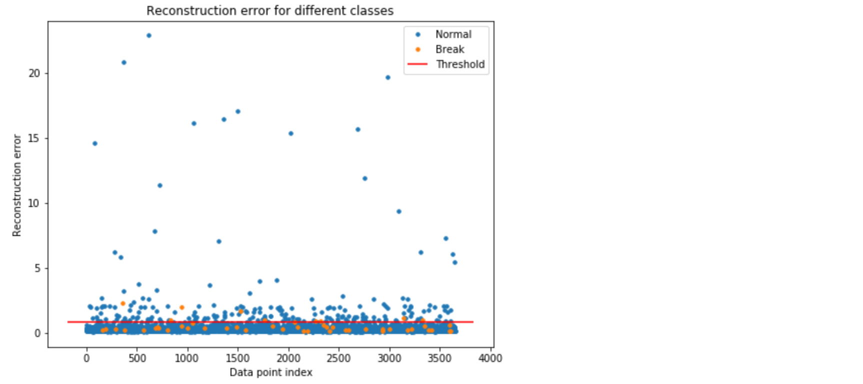
In Figure 4, the orange and blue dot above the threshold line represents the True Positive and False Positive, respectively. As we can see, we have good number of false positives.
Let’s see the accuracy results.
Test Accuracy
Confusion Matrix
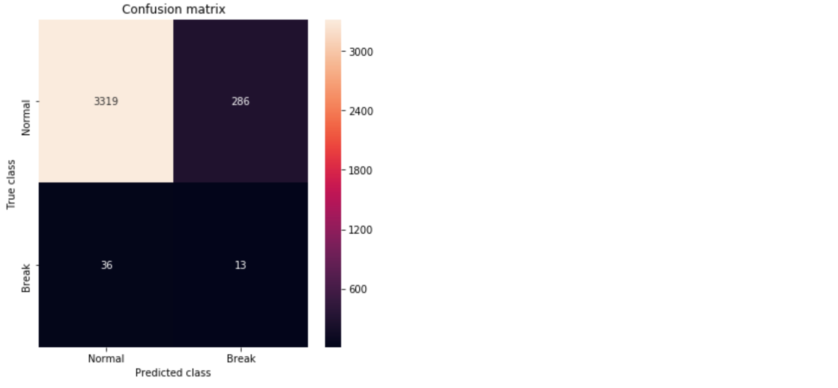
pred_y = [1 if e > threshold_fixed else 0 for e in error_df.Reconstruction_error.values]conf_matrix = confusion_matrix(error_df.True_class, pred_y)

plt.figure(figsize=(6, 6))
sns.heatmap(conf_matrix, xticklabels=LABELS, yticklabels=LABELS, annot=True, fmt="d");
plt.title("Confusion matrix")
plt.ylabel('True class')
plt.xlabel('Predicted class')
plt.show()

ROC Curve and AUC
false_pos_rate, true_pos_rate, thresholds = roc_curve(error_df.True_class, error_df.Reconstruction_error)
roc_auc = auc(false_pos_rate, true_pos_rate,)

plt.plot(false_pos_rate, true_pos_rate, linewidth=5, label='AUC = %0.3f'% roc_auc)
plt.plot([0,1],[0,1], linewidth=5)

plt.xlim([-0.01, 1])
plt.ylim([0, 1.01])
plt.legend(loc='lower right')
plt.title('Receiver operating characteristic curve (ROC)')
plt.ylabel('True Positive Rate')
plt.xlabel('False Positive Rate')
plt.show()

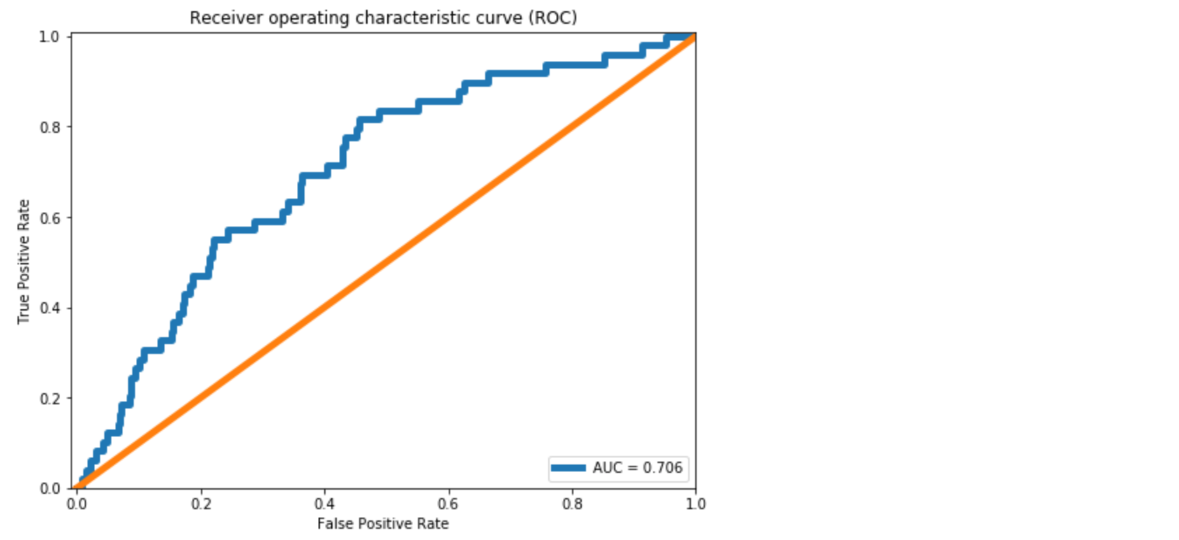
We see approximately 10% improvement in the AUC compared to the dense layer Autoencoder in [1]. From the Confusion Matrix in Figure 5, we could predict 10 out of 39 break instances. As also discussed in [1], this is significant for a paper mill. However, the improvement we achieved in comparison to the dense layer Autoencoder is minor.
The primary reason is LSTM model has more parameters to estimate. It becomes important to use regularization with LSTMs. Regularization and other model improvements will be discussed in the next post.
Github repository
cran2367/lstm_autoencoder_classifier
An LSTM Autoencoder for rare event classification. Contribute to cran2367/lstm_autoencoder_classifier development by…
github.com
What can be done better?
In the next article, we will learn tuning an Autoencoder. We will go over,
- CNN LSTM Autoencoder,
- Dropout layer,
- LSTM Dropout (Dropout_U and Dropout_W)
- Gaussian-dropout layer
- SELU activation, and
- alpha-dropout with SELU activation.
Conclusion
This post continued the work on extreme rare event binary labeled data in [1]. To utilize the temporal patterns, LSTM Autoencoders is used to build a rare event classifier for a multivariate time-series process. Details about the data preprocessing steps for LSTM model are discussed. A simple LSTM Autoencoder model is trained and used for classification. Some improvement in the accuracy over a Dense Autoencoder is found. For further improvement, we will look at ways to improve an Autoencoder with Dropout and other techniques in the next post.
[/vc_column_text][/vc_column][/vc_row][vc_row type=”in_container” full_screen_row_position=”middle” scene_position=”center” text_color=”dark” text_align=”left” top_padding=”20″ bottom_padding=”20″ overlay_strength=”0.3″ shape_divider_position=”bottom” bg_image_animation=”none” shape_type=””][vc_column column_padding=”no-extra-padding” column_padding_position=”all” background_color_opacity=”1″ background_hover_color_opacity=”1″ column_link_target=”_self” column_shadow=”none” column_border_radius=”none” width=”1/1″ tablet_width_inherit=”default” tablet_text_alignment=”default” phone_text_alignment=”default” column_border_width=”none” column_border_style=”solid” bg_image_animation=”none”][divider line_type=”Full Width Line” line_thickness=”1″ divider_color=”default”][/vc_column][/vc_row][vc_row type=”in_container” full_screen_row_position=”middle” scene_position=”center” text_color=”dark” text_align=”left” overlay_strength=”0.3″ shape_divider_position=”bottom” bg_image_animation=”none”][vc_column column_padding=”no-extra-padding” column_padding_position=”all” background_color_opacity=”1″ background_hover_color_opacity=”1″ column_link_target=”_self” column_shadow=”none” column_border_radius=”none” width=”1/1″ tablet_width_inherit=”default” tablet_text_alignment=”default” phone_text_alignment=”default” column_border_width=”none” column_border_style=”solid” bg_image_animation=”none”][vc_column_text]Originally posted on Medium.[/vc_column_text][/vc_column][/vc_row]