By: Chitta Ranjan, Ph.D., Director of Science, ProcessMiner, Inc.
In this case study, we will learn how to implement an autoencoder for building a rare-event classifier. We will use a real-world rare event dataset.
Background: What is an extreme rare event?
In a rare-event problem, we have an unbalanced dataset. Meaning, we have fewer positively labeled samples than negative. In a typical rare-event problem, the positively labeled data are around 5–10% of the total. In an extremely rare event problem, we have less than 1% positively labeled data. For example, in the dataset used here, it is around 0.6%.
Such extreme rare event problems are quite common in the real-world, for example, sheet-breaks and machine failure in manufacturing, clicks, or purchase in the online industry.
Classifying these rare events is quite challenging. Recently, Deep Learning has been quite extensively used for classification. However, the small number of positively labeled samples prohibits Deep Learning applications. No matter how large the data, the use of Deep Learning gets limited by the amount of positively labeled samples.
Why should we still bother to use Deep Learning?
This is a legitimate question. Why should we not think of using some another Machine Learning approach?
The answer is subjective. We can always go with a Machine Learning approach. To make it work, we can undersample from negatively labeled data to have a close to a balanced dataset. Since we have about 0.6% positively labeled data, the undersampling will result in rougly a dataset that is about 1% of the size of the original data. A Machine Learning approach, e.g. SVM or Random Forest, will still work on a dataset of this size. However, it will have limitations in its accuracy. And we will not utilize the information present in the remaining ~99% of the data.
If the data is sufficient, Deep Learning methods are potentially more capable. It also allows flexibility for model improvement by using different architectures. We will, therefore, attempt to use Deep Learning methods.
In this post, we will learn how we can use a simple dense layers autoencoder to build a rare event classifier. The purpose of this post is to demonstrate the implementation of an Autoencoder for extreme rare-event classification. We will leave the exploration of different architecture and configuration of the Autoencoder on the user. Please share in the comments if you find anything interesting.
Autoencoder for Classification
The autoencoder approach for classification is similar to anomaly detection. In anomaly detection, we learn the pattern of a normal process. Anything that does not follow this pattern is classified as an anomaly. For a binary classification of rare events, we can use a similar approach using autoencoders (derived from here [2]).
Quick revision: What is an autoencoder?
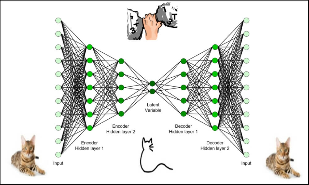
- An autoencoder is made of two modules: encoder and decoder
- The encoder learns the underlying features of a process; these features are typically in a reduced dimension
- The decoder can recreate the original data from these underlying features
How to use an Autoencoder rare-event classification?
- We will divide the data into two parts: positively labeled and negatively labeled
- The negatively labeled data is treated as a normal state of the process; A normal state is when the process is relentless
- We will ignore the positively labeled data, and train an Autoencoder on only negatively labeled data
- This Autoencoder has now learned the features of the normal process
- A well-trained Autoencoder will predict any new data that is coming from the normal state of the process (as it will have the same pattern or distribution)
- Therefore, the reconstruction error will be small
- However, if we try to reconstruct data from a rare-event, the Autoencoder will struggle
- This will make the reconstruction error high during the rare-event
- We can catch such high reconstruction errors and label them as a rare-event prediction
- This procedure is similar to anomaly detection methods
Implementation: Data and Problem
This is a binary labeled data from a pulp-and-paper mill for sheet breaks. Sheet breaks is a severe problem in paper manufacturing. A single sheet break causes a loss of several thousand dollars, and the mills see at least one or more breaks every day. This causes millions of dollars of yearly losses and work hazards.
Detecting a break event is challenging due to the nature of the process. As mentioned in [1], even a 5% reduction in the breaks will bring significant benefit to the mills.
The data we have contains about 18k rows collected over 15 days. The column contains the binary labels, with 1 denoting a sheet break. The rest columns are predictors. There are about 124 positive labeled samples (~0.6%).
Code: Import the desired libraries.
%matplotlib inline
import matplotlib.pyplot as plt
import seaborn as snsimport pandas as pd
import numpy as np
from pylab import rcParamsimport tensorflow as tf
from keras.models import Model, load_model
from keras.layers import Input, Dense
from keras.callbacks import ModelCheckpoint, TensorBoard
from keras import regularizersfrom sklearn.preprocessing import StandardScaler
from sklearn.model_selection import train_test_split
from sklearn.metrics import confusion_matrix, precision_recall_curve
from sklearn.metrics import recall_score, classification_report, auc, roc_curve
from sklearn.metrics import precision_recall_fscore_support, f1_scorefrom numpy.random import seed
seed(1)
from tensorflow import set_random_seed
set_random_seed(2)SEED = 123 #used to help randomly select the data points
DATA_SPLIT_PCT = 0.2rcParams['figure.figsize'] = 8, 6
LABELS = ["Normal","Break"]
Note that we are setting the random seeds for the reproducibility of the result.
Data Preprocessing
Now, we read and prepare the data.[/vc_column_text][vc_column_text]
df = pd.read_csv("data/processminer-rare-event-mts - data.csv")
The objective of this rare-event problem is to predict a sheet-break before it occurs. We will try to predict the break 4 minutes in advance. To build this model, we will shift the labels 2 rows up (which corresponds to 4 minutes). We can do this as: However, in this problem, we would want to do the shifting as: if row n is positively labeled:
- make rows (n-2) and (n-1) equal to 1 | This will help the classifier learn up to 4 minutes ahead prediction
- Delete row n, bsecause we do not want the classifier to learn to predict a break when it has happened
We will develop the following UDF for this curve shifting.[/vc_column_text][vc_column_text]
sign = lambda x: (1, -1)[x < 0]

def curve_shift(df, shift_by):
    '''
    This function will shift the binary labels in a dataframe.
    The curve shift will be with respect to the 1s.
    For example, if shift is -2, the following process
    will happen: if row n is labeled as 1, then
    - Make row (n+shift_by):(n+shift_by-1) = 1.
    - Remove row n.
    i.e. the labels will be shifted up to 2 rows up.

    Inputs:
    df       A pandas dataframe with a binary labeled column.
             This labeled column should be named as 'y'.
    shift_by An integer denoting the number of rows to shift.

    Output
    df       A dataframe with the binary labels shifted by shift.
    '''

    vector = df['y'].copy()
    for s in range(abs(shift_by)):
        tmp = vector.shift(sign(shift_by))
        tmp = tmp.fillna(0)
        vector += tmp
    labelcol = 'y'
    # Add vector to the df
    df.insert(loc=0, column=labelcol+'tmp', value=vector)
    # Remove the rows with labelcol == 1.
    df = df.drop(df[df[labelcol] == 1].index)
    # Drop labelcol and rename the tmp col as labelcol
    df = df.drop(labelcol, axis=1)
    df = df.rename(columns={labelcol+'tmp': labelcol})
    # Make the labelcol binary
    df.loc[df[labelcol] > 0, labelcol] = 1

    return df
Before moving forward, we will drop the time, and also the categorical columns for simplicity.
# Remove time column, and the categorical columns
df = df.drop(['time', 'x28', 'x61'], axis=1)
Now, we divide the data into train, valid, and test sets. Then we will take the subset of data with only 0s to train the autoencoder.
df_train, df_test = train_test_split(df, test_size=DATA_SPLIT_PCT, random_state=SEED)
df_train, df_valid = train_test_split(df_train, test_size=DATA_SPLIT_PCT, random_state=SEED)df_train_0 = df_train.loc[df['y'] == 0]
df_train_1 = df_train.loc[df['y'] == 1]
df_train_0_x = df_train_0.drop(['y'], axis=1)
df_train_1_x = df_train_1.drop(['y'], axis=1)df_valid_0 = df_valid.loc[df['y'] == 0]
df_valid_1 = df_valid.loc[df['y'] == 1]
df_valid_0_x = df_valid_0.drop(['y'], axis=1)
df_valid_1_x = df_valid_1.drop(['y'], axis=1)df_test_0 = df_test.loc[df['y'] == 0]
df_test_1 = df_test.loc[df['y'] == 1]
df_test_0_x = df_test_0.drop(['y'], axis=1)
df_test_1_x = df_test_1.drop(['y'], axis=1)
Standardization: It is usually better to use standardized data (transformed to Gaussian, mean 0 and variance 1) for autoencoders.
scaler = StandardScaler().fit(df_train_0_x)
df_train_0_x_rescaled = scaler.transform(df_train_0_x)
df_valid_0_x_rescaled = scaler.transform(df_valid_0_x)
df_valid_x_rescaled = scaler.transform(df_valid.drop(['y'], axis = 1))df_test_0_x_rescaled = scaler.transform(df_test_0_x)
df_test_x_rescaled = scaler.transform(df_test.drop(['y'], axis = 1))
Autoencoder Classifier
Initialization: First, we will initialize Autoencoder architecture. We are building a simple autoencoder. More complex architectures and other configurations should be explored.
nb_epoch = 200
batch_size = 128
input_dim = df_train_0_x_rescaled.shape[1] #num of predictor variables,
encoding_dim = 32
hidden_dim = int(encoding_dim / 2)
learning_rate = 1e-3

input_layer = Input(shape=(input_dim, ))
encoder = Dense(encoding_dim, activation="relu", activity_regularizer=regularizers.l1(learning_rate))(input_layer)
encoder = Dense(hidden_dim, activation="relu")(encoder)
decoder = Dense(hidden_dim, activation="relu")(encoder)
decoder = Dense(encoding_dim, activation="relu")(decoder)
decoder = Dense(input_dim, activation="linear")(decoder)
autoencoder = Model(inputs=input_layer, outputs=decoder)
autoencoder.summary()
Training: We will train the model and save it in a file. Saving a trained model is a good practice for saving time for future analysis.
autoencoder.compile(metrics=['accuracy'],
                    loss='mean_squared_error',
                    optimizer='adam')cp = ModelCheckpoint(filepath="autoencoder_classifier.h5",
                               save_best_only=True,
                               verbose=0)tb = TensorBoard(log_dir='./logs',
                histogram_freq=0,
                write_graph=True,
                write_images=True)history = autoencoder.fit(df_train_0_x_rescaled, df_train_0_x_rescaled,
                    epochs=nb_epoch,
                    batch_size=batch_size,
                    shuffle=True,
                    validation_data=(df_valid_0_x_rescaled, df_valid_0_x_rescaled),
                    verbose=1,
                    callbacks=[cp, tb]).history
Classification: In the following, we show how we can use an Autoencoder reconstruction error for the rare-event classification.
As mentioned before, if the reconstruction error is high, we will classify it as a sheet-break. We will need to determine the threshold for this.
We will use the validation set to identify the threshold.
valid_x_predictions = autoencoder.predict(df_valid_x_rescaled)
mse = np.mean(np.power(df_valid_x_rescaled - valid_x_predictions, 2), axis=1)
error_df = pd.DataFrame({'Reconstruction_error': mse,
                        'True_class': df_valid['y']})precision_rt, recall_rt, threshold_rt = precision_recall_curve(error_df.True_class, error_df.Reconstruction_error)
plt.plot(threshold_rt, precision_rt[1:], label="Precision",linewidth=5)
plt.plot(threshold_rt, recall_rt[1:], label="Recall",linewidth=5)
plt.title('Precision and recall for different threshold values')
plt.xlabel('Threshold')
plt.ylabel('Precision/Recall')
plt.legend()
plt.show()
We should not estimate the classification threshold from the test data. It will result in overfitting.
test_x_predictions = autoencoder.predict(df_test_x_rescaled)
mse = np.mean(np.power(df_test_x_rescaled - test_x_predictions, 2), axis=1)
error_df_test = pd.DataFrame({'Reconstruction_error': mse,
                        'True_class': df_test['y']})
error_df_test = error_df_test.reset_index()threshold_fixed = 0.4
groups = error_df_test.groupby('True_class')fig, ax = plt.subplots()for name, group in groups:
    ax.plot(group.index, group.Reconstruction_error, marker='o', ms=3.5, linestyle='',
            label= "Break" if name == 1 else "Normal")
ax.hlines(threshold_fixed, ax.get_xlim()[0], ax.get_xlim()[1], colors="r", zorder=100, label='Threshold')
ax.legend()
plt.title("Reconstruction error for different classes")
plt.ylabel("Reconstruction error")
plt.xlabel("Data point index")
plt.show();
pred_y = [1 if e > threshold_fixed else 0 for e in error_df.Reconstruction_error.values]conf_matrix = confusion_matrix(error_df.True_class, pred_y)plt.figure(figsize=(12, 12))
sns.heatmap(conf_matrix, xticklabels=LABELS, yticklabels=LABELS, annot=True, fmt="d");
plt.title("Confusion matrix")
plt.ylabel('True class')
plt.xlabel('Predicted class')
plt.show()
We could predict 8 out of 41 breaks instances. Note that these instances include 2 or 4 minute ahead predictions. This is around 20%, which is a good recall rate for the paper industry. The False Positive Rate is around 6%. This is not ideal but not terrible for a mill.
Still, this model can be further improved to increase the recall rate with smaller False Positive Rate. We will look at the AUC below and then talk about the next approach for improvement.
ROC Curve and AUC
false_pos_rate, true_pos_rate, thresholds = roc_curve(error_df.True_class, error_df.Reconstruction_error)
roc_auc = auc(false_pos_rate, true_pos_rate,)plt.plot(false_pos_rate, true_pos_rate, linewidth=5, label='AUC = %0.3f'% roc_auc)
plt.plot([0,1],[0,1], linewidth=5)plt.xlim([-0.01, 1])
plt.ylim([0, 1.01])
plt.legend(loc='lower right')
plt.title('Receiver operating characteristic curve (ROC)')
plt.ylabel('True Positive Rate')
plt.xlabel('False Positive Rate')
plt.show()
Github Repository
The entire code with comments is present here.
cran2367/autoencoder_classifier
Autoencoder model for rare event classification. Contribute to cran2367/autoencoder_classifier development by creating…
github.com
What Can Be Done Better Here?
Autoencoder Optimization
Autoencoders are a nonlinear extension of PCA. However, the conventional Autoencoder developed above does not follow the principles of PCA. In Build the right Autoencoder — Tune and Optimize using PCA principles. Part I and Part II, the required PCA principles that should be incorporated in an Autoencoder for optimization are explained and implemented.
LSTM Autoencoder
The problem discussed here is a (multivariate) time series. However, in the Autoencoder model, we are not taking into account the temporal information/patterns. In the next post, we will explore if it is possible with an RNN. We will try an LSTM autoencoder.
Conclusion
We worked on an extreme rare event binary labeled data from a paper mill to build an Autoencoder Classifier. We achieved reasonable accuracy. The purpose here was to demonstrate the use of a basic Autoencoder for rare event classification. We will further work on developing other methods, including an LSTM Autoencoder that can extract the temporal features for better accuracy.