

The evolution of statistical process monitoring
Title: The Evolution and Required Transformation of Statistical Process Monitoring
By Bill Woodall, Professor Emeritus of Statistics, Virginia Tech | Originally published Oct 20, 2021 | Technology
In Industry 4.0, there is a need for automated diagnosis of process monitoring alarms along with root cause determination and process adjustment. Computationally intensive and adaptable approaches such as those incorporated into ProcessMiner software are required for these reasons.
Our readers are likely familiar with the industrial practice being broken down into the following four roughly defined eras: Industry 1.0 (use of water and steam power and mechanization starting about 1800), Industry 2.0 (use of electricity, mass production, and assembly lines starting about 1900), Industry 3.0 (use of automation and information technology starting about 1970) and now Industry 4.0 (use of cyber-physical control and big data starting about 2011). In addition to advances in technology, these eras of industrial practice could also be characterized in terms of increases in the availability and use of data.
Industry 2.0 and Statistical Process Monitoring
Statistical process monitoring (SPM) originated with Walter Shewhart’s work at Western Electric during the Industry 2.0 era. Shewhart was the first person to recognize that the time order of industrial data could be very informative. Data collection was slow, manual, and expensive in his day. Sampling frequencies were typically low. The first Shewhart chart in 1924, for example, involved a plot of proportions of non-conforming items with the data aggregated over months. Any calculations had to be simplified in order to be done by hand. The Shewhart control limits were set at plus and minus three standard deviations of the control chart statistic from the centerline. The Western Electric Handbook, which operationalized Shewhart’s ideas, was first published in 1956.
There were some major advances in SPM methods during Industry 2.0. Harold Hotelling introduced the first chart for monitoring multivariate data in 1947. S. W. Roberts introduced the exponentially weighted moving average (EWMA) chart in 1959 and E. S. Page introduced the cumulative sum (CUSUM) chart in 1961. These methods made better use of information in recent data. It does not seem, however, that the EWMA and CUSUM methods had much of an influence on industrial practice in this era.
Richard Freund of Kodak introduced the acceptance control chart in 1957. The purpose of his chart was to widen the Shewhart chart control limits to avoid the detection of process shifts that were considered to be too small to be of practical importance.
As another notable contribution, in 1959 J. E. Jackson proposed a multivariate monitoring method based on the use of principal components. It was much later, however, before the principal component methods could be used to their full potential.
Industry 3.0 and Statistical Process Monitoring
The quality revolution in the U.S. started around 1980, well into the Industry 3.0 era. The primary driving force behind the quality revolution was quality and price competition from Japanese companies. Statistical monitoring methods became widely used and in some cases oversold. W. E. Deming was the de facto spiritual leader of the quality revolution because much of the Japanese quality success was attributed to his teaching in Japan in 1950 and later. Deming was a strong proponent of process improvement by continual variation reduction. He also advocated the use of the Shewhart control chart, writing that no method of monitoring was better. In particular, he was opposed to the widening of the Shewhart three-sigma control limits.
As the amount of data increased during Industry 3.0, more and more SPM methods were developed. Computation became much less of an issue with software, such as Minitab® and JMP®, becoming available. There were additional multivariate methods introduced such as the multivariate EWMA chart and multivariate CUSUM charts. As sampling frequencies increased, it became important to account for autocorrelation in the data. Manufacturing processes are almost invariably multi-stage, so methods were developed to account for incoming quality, not just outgoing process quality, at each stage.
Methods were developed in Industry 3.0 for monitoring processes where there was more than just the one variance component assumed with Shewhart control charts. For example, with batch data, there could be variation between batches as well as variation within batches. There were extensions required for the monitoring of functional data (called profile monitoring), where quality is best characterized by a relationship between a response variable and one or more explanatory variables. One of the first applications of profile monitoring was developed at the U.S. National Bureau of Standards for monitoring calibration curves. Some methods were also developed for monitoring image and video data.
Industry 4.0 and Statistical Process Monitoring
Although standard Industry 2.0 and 3.0 statistical process monitoring methods can remain useful, they fail to work well, if at all, in many Industry 4.0 applications. Industry 4.0 data are often high-dimensional with high sampling frequencies. Control charts have been developed to signal for data that indicated a statistically significant process change. With massive amounts of data, any change, however small, becomes statistically significant. In an increasing number of cases, the focus needs to be on detecting, to the extent possible, only process changes of practical importance. In effect, control charts and warning systems, in general, need to be tuned to detect shifts of practical interest, which will vary by application.
Having a smoke alarm that is activated by the striking of a match would be very undesirable in a kitchen, for example, but such sensitivity might be desirable in an airplane lavatory. Thus, there needs to be a return to some of the basic ideas of Richard Freund and the acceptance control chart. The focus needs to be on the practical importance, not just the statistical significance, of process changes.
There are other complicating issues that can arise with Industry 4.0 data. The use of sensor technology leads to high dimensional data, so dimension reduction methods can be helpful to take advantage of the resulting duplication of information. The high sampling frequencies require decisions about the appropriate level of data aggregation. Sampling frequencies will rarely be synchronized for the measured variables, as assumed in Industry 3.0 multivariate methods. In particular, quality variables are often measured at much lower frequencies than process variables and are often characterized by delays such as those due to lab work.
The types of data in Industry 4.0 can vary as well with attribute data, variables data, profiles and image data all required for decision making. In addition, there can be complicated relationships between variables involving correlation and causation.
The data involved in Industry 4.0 applications can be far too complicated to be handled by traditional statistical process monitoring approaches. Modeling and using the process data effectively, even by process experts, is often impossible. That is precisely the kind of automated diagnosis and root cause determination that computationally intensive, adaptable approaches — including software such as ProcessMiner’s — are built to provide.
LSTM autoencoder for anomaly detection in Keras
By: Chitta Ranjan, Ph.D., Director of Science, ProcessMiner, Inc.
Here we will learn the details of data preparation for LSTM models, and build an LSTM Autoencoder for rare-event classification.
This post is a continuation of my previous post Extreme Rare Event Classification using Autoencoders. In the previous post, we talked about the challenges in an extremely rare event data with less than 1% positively labeled data. We built an Autoencoder Classifier for such processes using the concepts of Anomaly Detection.
However, the data we have is a time series. But earlier we used a Dense layer Autoencoder that does not use the temporal features in the data. Therefore, in this post, we will improve on our approach by building an LSTM Autoencoder.
Here, we will learn:
- data preparation steps for an LSTM model,
- building and implementing LSTM autoencoder, and
- using LSTM autoencoder for rare-event classification.
Quick recap on LSTM:
- LSTM is a type of Recurrent Neural Network (RNN). RNNs, in general, and LSTM, specifically, are used on sequential or time series data.
- These models are capable of automatically extracting effect of past events.
- LSTM are known for its ability to extract both long- and short- term effects of pasts event.
In the following, we will go directly to developing an LSTM Autoencoder. It is recommended to read Step-by-step understanding LSTM Autoencoder layers to better understand and further improve the network below.
About the data problem in brief, we have real-world data on sheet breaks from a paper manufacturing. Our objective is to predict the break in advance. Please refer to Extreme Rare Event Classification using Autoencoders for the details on the data, problem, and the classification approach.
LSTM Autoencoder for Multivariate Data
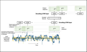 Figure 1. An LSTM Autoencoder.
In our problem, we have a multivariate time-series data. A multivariate time-series data contains multiple variables observed over a period of time. We will build an LSTM autoencoder on this multivariate time-series to perform rare-event classification. As described in [1], this is achieved by using an anomaly detection approach:
- we build an autoencoder on the normal (negatively labeled) data,
- use it to reconstruct a new sample,
- if the reconstruction error is high, we label it as a sheet-break.
LSTM requires few special data-preprocessing steps. In the following, we will give sufficient attention to these steps.
Let’s get to the implementation.
Libraries
I like to put together the libraries and global constants first.
%matplotlib inline
import matplotlib.pyplot as plt
import seaborn as sns

import pandas as pd
import numpy as np
from pylab import rcParams

import tensorflow as tf
from keras import optimizers, Sequential
from keras.models import Model
from keras.utils import plot_model
from keras.layers import Dense, LSTM, RepeatVector, TimeDistributed
from keras.callbacks import ModelCheckpoint, TensorBoard

from sklearn.preprocessing import StandardScaler
from sklearn.model_selection import train_test_split
from sklearn.metrics import confusion_matrix, precision_recall_curve
from sklearn.metrics import recall_score, classification_report, auc, roc_curve
from sklearn.metrics import precision_recall_fscore_support, f1_score

from numpy.random import seed
seed(7)
from tensorflow import set_random_seed
set_random_seed(11)from sklearn.model_selection import train_test_split

SEED = 123 #used to help randomly select the data points
DATA_SPLIT_PCT = 0.2

rcParams['figure.figsize'] = 8, 6
LABELS = ["Normal","Break"]
Data Preparation
As mentioned before, LSTM requires a few specific steps in the data preparation. The input to LSTMs are 3-dimensional arrays created from the time-series data. This is an error prone step so we will look at the details.
Read data
The data is taken from [2]. The link to the data is here.
df = pd.read_csv("data/processminer-rare-event-mts - data.csv")
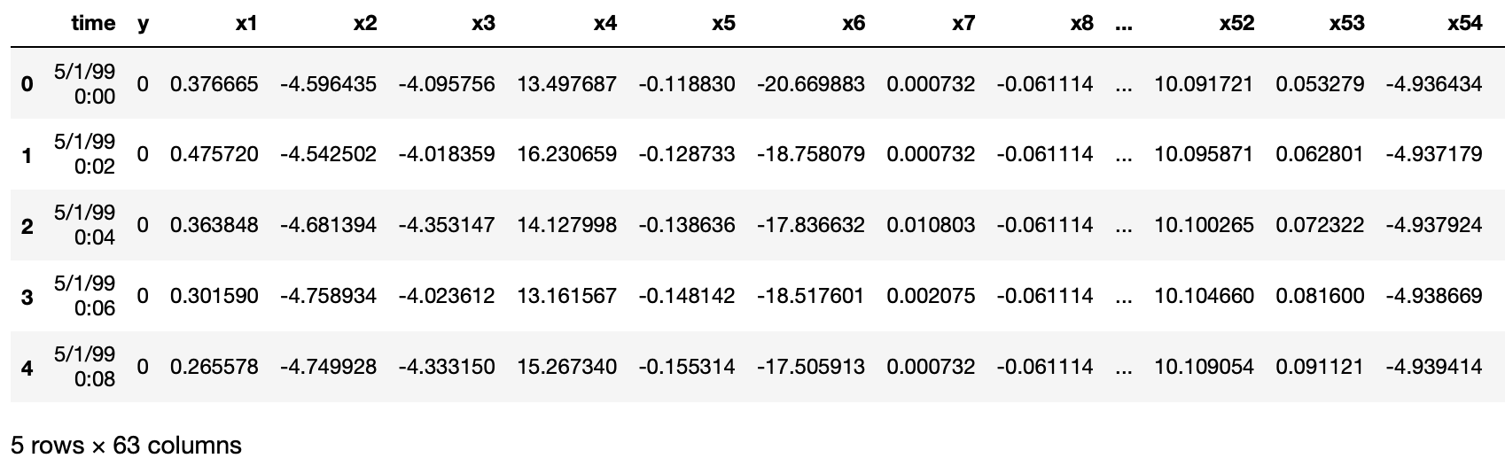
df.head(n=5)  # visualize the data.
Curve Shifting
As also mentioned in [1], the objective of this rare-event problem is to predict a sheet-break before it occurs. We will try to predict the break up to 4 minutes in advance. For this data, this is equivalent to shifting the labels up by two rows. It can be done directly with df.y=df.y.shift(-2). However, here we require to do the following,
- For any row n with label 1, make (n-2):(n-1) as 1. With this, we are teaching the classifier to predict up to 4 minutes ahead. And,
- remove row n. Row n is removed because we are not interested in teaching the classifier to predict a break when it has already happened.
We develop the following function to perform this curve shifting.
sign = lambda x: (1, -1)[x < 0]

def curve_shift(df, shift_by):
    '''
    This function will shift the binary labels in a dataframe.
    The curve shift will be with respect to the 1s.
    For example, if shift is -2, the following process
    will happen: if row n is labeled as 1, then
    - Make row (n+shift_by):(n+shift_by-1) = 1.
    - Remove row n.
    i.e. the labels will be shifted up to 2 rows up.

    Inputs:
    df       A pandas dataframe with a binary labeled column.
             This labeled column should be named as 'y'.
    shift_by An integer denoting the number of rows to shift.

    Output
    df       A dataframe with the binary labels shifted by shift.
    '''

    vector = df['y'].copy()
    for s in range(abs(shift_by)):
        tmp = vector.shift(sign(shift_by))
        tmp = tmp.fillna(0)
        vector += tmp
    labelcol = 'y'
    # Add vector to the df
    df.insert(loc=0, column=labelcol+'tmp', value=vector)
    # Remove the rows with labelcol == 1.
    df = df.drop(df[df[labelcol] == 1].index)
    # Drop labelcol and rename the tmp col as labelcol
    df = df.drop(labelcol, axis=1)
    df = df.rename(columns={labelcol+'tmp': labelcol})
    # Make the labelcol binary
    df.loc[df[labelcol] > 0, labelcol] = 1

    return df
We will now shift our data and verify if the shifting is correct. In the subsequent sections, we have few more test steps. It is recommended to use them to ensure the data preparation steps are working as expected.
print('Before shifting')  # Positive labeled rows before shifting.
one_indexes = df.index[df['y'] == 1]
display(df.iloc[(np.where(np.array(input_y) == 1)[0][0]-5):(np.where(np.array(input_y) == 1)[0][0]+1), ])

# Shift the response column y by 2 rows to do a 4-min ahead prediction.
df = curve_shift(df, shift_by = -2)

print('After shifting')  # Validating if the shift happened correctly.
display(df.iloc[(one_indexes[0]-4):(one_indexes[0]+1), 0:5].head(n=5))
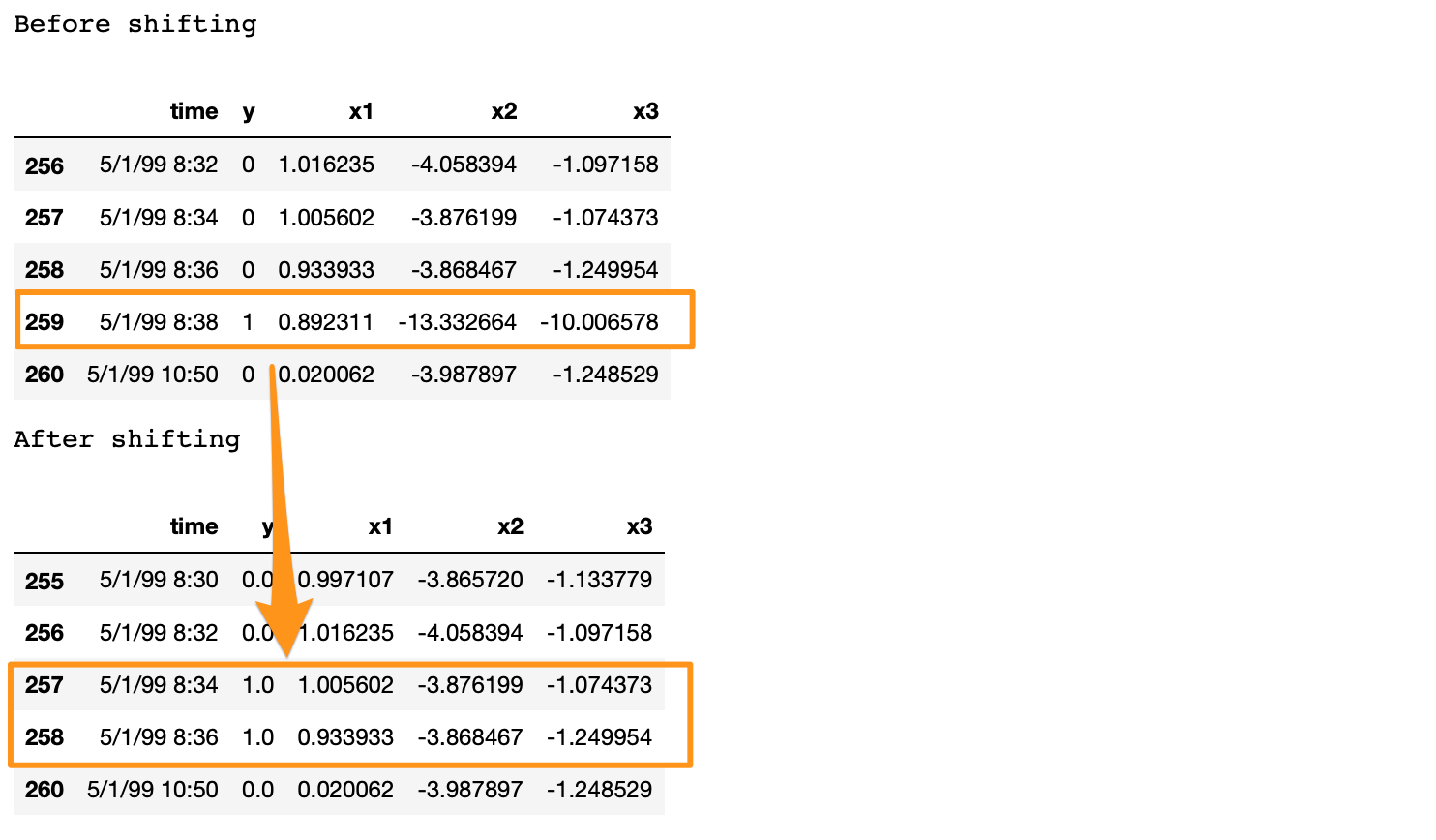
If we note here, we moved the positive label at 5/1/99 8:38 to n-1 and n-2 timestamps, and dropped row n. Also, there is a time difference of more than 2 minutes between a break row and the next row. This is because, when a break occurs, the machine stays in the break status for a while. During this time, we have y = 1 for consecutive rows. In the provided data, these consecutive break rows are deleted to prevent the classifier from learning to predict a break after it has already happened. Refer [2] for details.
Before moving forward, we clean up the data by dropping the time, and two other categorical columns.
# Remove time column, and the categorical columns
df = df.drop(['time', 'x28', 'x61'], axis=1)
Prepare Input Data for LSTM
LSTM is a bit more demanding than other models. Significant amount of time and attention may go in preparing the data that fits an LSTM. However, it is generally worth the effort.
The input data to an LSTM model is a 3-dimensional array. The shape of the array is samples x lookback x features. Let’s understand them,
- samples: This is simply the number of observations, or in other words, the number of data points.
- lookback: LSTM models are meant to look at the past. Meaning, at time t the LSTM will process data up to (t–lookback) to make a prediction.
- features: It is the number of features present in the input data.
First, we will extract the features and response.
input_X = df.loc[:, df.columns != 'y'].values  # converts the df to a numpy array
input_y = df['y'].values

n_features = input_X.shape[1]  # number of features
The input_X here is a 2-dimensional array of size samples x features. We want to be able to transform such a 2D array into a 3D array of size: samples x lookback x features. Refer to Figure 1 above for a visual understanding.
For that, we develop a function temporalize .
def temporalize(X, y, lookback):
    '''
    Inputs
    X         A 2D numpy array ordered by time of shape:
              (n_observations x n_features)
    y         A 1D numpy array with indexes aligned with
              X, i.e. y[i] should correspond to X[i].
              Shape: n_observations.
    lookback  The window size to look back in the past
              records. Shape: a scalar.

    Output
    output_X  A 3D numpy array of shape:
              ((n_observations-lookback-1) x lookback x
              n_features)
    output_y  A 1D array of shape:
              (n_observations-lookback-1), aligned with X.
    '''
    output_X = []
    output_y = []
    for i in range(len(X) - lookback - 1):
        t = []
        for j in range(1, lookback + 1):
            # Gather the past records upto the lookback period
            t.append(X[[(i + j + 1)], :])
        output_X.append(t)
        output_y.append(y[i + lookback + 1])
    return np.squeeze(np.array(output_X)), np.array(output_y)
To test and demonstrate this function, we will look at an example below with lookback = 5 .
print('First instance of y = 1 in the original data')
display(df.iloc[(np.where(np.array(input_y) == 1)[0][0]-5):(np.where(np.array(input_y) == 1)[0][0]+1), ])lookback = 5  # Equivalent to 10 min of past data.
# Temporalize the data
X, y = temporalize(X = input_X, y = input_y, lookback = lookback)print('For the same instance of y = 1, we are keeping past 5 samples in the 3D predictor array, X.')
display(pd.DataFrame(np.concatenate(X[np.where(np.array(y) == 1)[0][0]], axis=0 )))
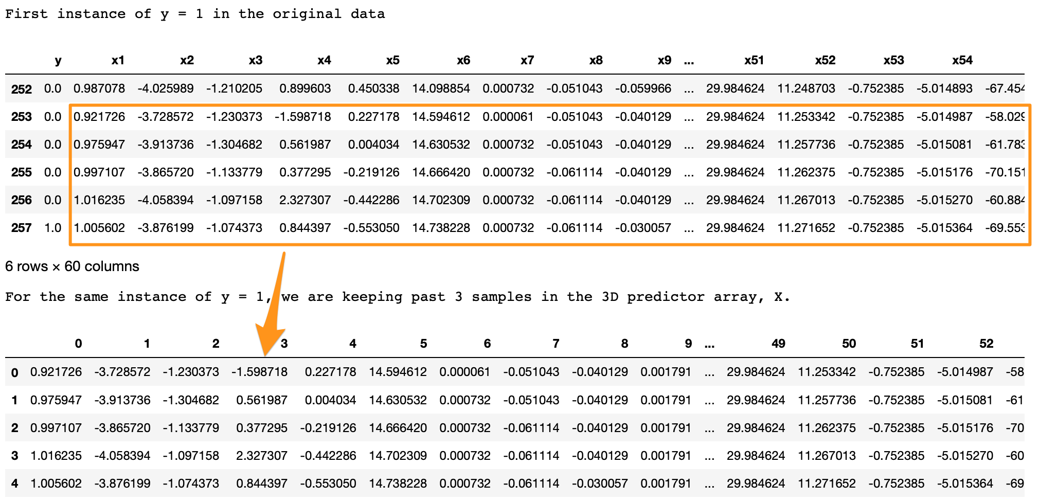
What we are looking for here is,
- In the original data, y = 1 at row 257.
- With
lookback = 5we want the LSTM to look at the 5 rows before row 257 (including itself). - In the 3D array,
X, each 2D block atX[i,:,:]denotes the prediction data that corresponds toy[i]. To draw an analogy, in regressiony[i]corresponds to a 1D vectorX[i,:]; in LSTMy[i]corresponds to a 2D arrayX[i,:,:]. - This 2D block
X[i,:,:]should have the predictors atinput_X[i,:]and the previous rows up to the givenlookback. - As we can see in the output above, the
X[i,:,:]block in the bottom is the same as the five past rows of y=1 shown on the top. - Similarly, this is applied for the entire data, for all y’s. The example here is shown for an instance of y=1 for easier visualization.
Split into train, valid, and test
This is straightforward with the sklearn function.
X_train, X_test, y_train, y_test = train_test_split(np.array(X), np.array(y), test_size=DATA_SPLIT_PCT, random_state=SEED)X_train, X_valid, y_train, y_valid = train_test_split(X_train, y_train, test_size=DATA_SPLIT_PCT, random_state=SEED)
For training the autoencoder, we will be using the X coming from only the negatively labeled data. Therefore, we separate the X corresponding to y = 0.
X_train_y0 = X_train[y_train==0]
X_train_y1 = X_train[y_train==1]X_valid_y0 = X_valid[y_valid==0]
X_valid_y1 = X_valid[y_valid==1]
We will reshape the X’s into the required 3D dimension: sample x lookback x features.
X_train = X_train.reshape(X_train.shape[0], lookback, n_features)
X_train_y0 = X_train_y0.reshape(X_train_y0.shape[0], lookback, n_features)
X_train_y1 = X_train_y1.reshape(X_train_y1.shape[0], lookback, n_features)X_valid = X_valid.reshape(X_valid.shape[0], lookback, n_features)
X_valid_y0 = X_valid_y0.reshape(X_valid_y0.shape[0], lookback, n_features)
X_valid_y1 = X_valid_y1.reshape(X_valid_y1.shape[0], lookback, n_features)X_test = X_test.reshape(X_test.shape[0], lookback, n_features)
Standardize the Data
It is usually better to use a standardized data (transformed to Gaussian with mean 0 and standard deviation 1) for autoencoders.
One common standardization mistake is: we normalize the entire data and then split into train-test. This is incorrect. Test data should be completely unseen to anything during the modeling. We should, therefore, normalize the training data, and use its summary statistics to normalize the test data (for normalization, these statistics are the mean and variances of each feature).
Standardizing this data is a bit tricky. This is because the X matrices are 3D, and we want the standardization to happen with respect to the original 2D data.
To do this, we will require two UDFs.
flatten: This function will re-create the original 2D array from which the 3D arrays were created. This function is the inverse oftemporalize, meaningX = flatten(temporalize(X)).scale: This function will scale a 3D array that we created as inputs to the LSTM.
def flatten(X):
    '''
    Flatten a 3D array.

    Input
    X            A 3D array for lstm, where the array is sample x timesteps x features.

    Output
    flattened_X  A 2D array, sample x features.
    '''
    flattened_X = np.empty((X.shape[0], X.shape[2]))  # sample x features array.
    for i in range(X.shape[0]):
        flattened_X[i] = X[i, (X.shape[1]-1), :]
    return(flattened_X)

def scale(X, scaler):
    '''
    Scale 3D array.

    Inputs
    X            A 3D array for lstm, where the array is sample x timesteps x features.
    scaler       A scaler object, e.g., sklearn.preprocessing.StandardScaler, sklearn.preprocessing.normalize

    Output
    X            Scaled 3D array.
    '''
    for i in range(X.shape[0]):
        X[i, :, :] = scaler.transform(X[i, :, :])

    return X
Why didn’t we first normalize the original 2D data and then create the 3D arrays? Because, to do this we will: split the data into train and test, followed by their normalization. However, when we create the 3D arrays on the test data, we lose the initial rows of samples up till the lookback. Splitting into train-valid-test will cause this for both the validation and test sets.
We will fit a Standardization object from sklearn. This function standardizes the data to Normal(0, 1). Note that we require to flatten the X_train_y0 array to pass to the fit function.
# Initialize a scaler using the training data.
scaler = StandardScaler().fit(flatten(X_train_y0))
We will use our UDF, scale, to standardize X_train_y0 with the fitted transform object scaler.
X_train_y0_scaled = scale(X_train_y0, scaler)
Make sure the scale worked correctly?
A correct transformation of X_train will ensure that the means and variances of each column of the flattened X_train are 0 and 1, respectively. We test this.
a = flatten(X_train_y0_scaled)
print('colwise mean', np.mean(a, axis=0).round(6))
print('colwise variance', np.var(a, axis=0))

All the means and variances outputted above are 0 and 1, respectively. Therefore, the scaling is correct. We will now scale the validation and test sets. We will again use the scaler object on these sets.
X_valid_scaled = scale(X_valid, scaler)
X_valid_y0_scaled = scale(X_valid_y0, scaler)X_test_scaled = scale(X_test, scaler)
LSTM Autoencoder Training
We will, first, initialize few variables.
timesteps =  X_train_y0_scaled.shape[1] # equal to the lookback
n_features =  X_train_y0_scaled.shape[2] # 59

epochs = 200
batch = 64
lr = 0.0001
We, now, develop a simple architecture.
lstm_autoencoder = Sequential()
# Encoder
lstm_autoencoder.add(LSTM(32, activation='relu', input_shape=(timesteps, n_features), return_sequences=True))
lstm_autoencoder.add(LSTM(16, activation='relu', return_sequences=False))
lstm_autoencoder.add(RepeatVector(timesteps))
# Decoder
lstm_autoencoder.add(LSTM(16, activation='relu', return_sequences=True))
lstm_autoencoder.add(LSTM(32, activation='relu', return_sequences=True))
lstm_autoencoder.add(TimeDistributed(Dense(n_features)))

lstm_autoencoder.summary()
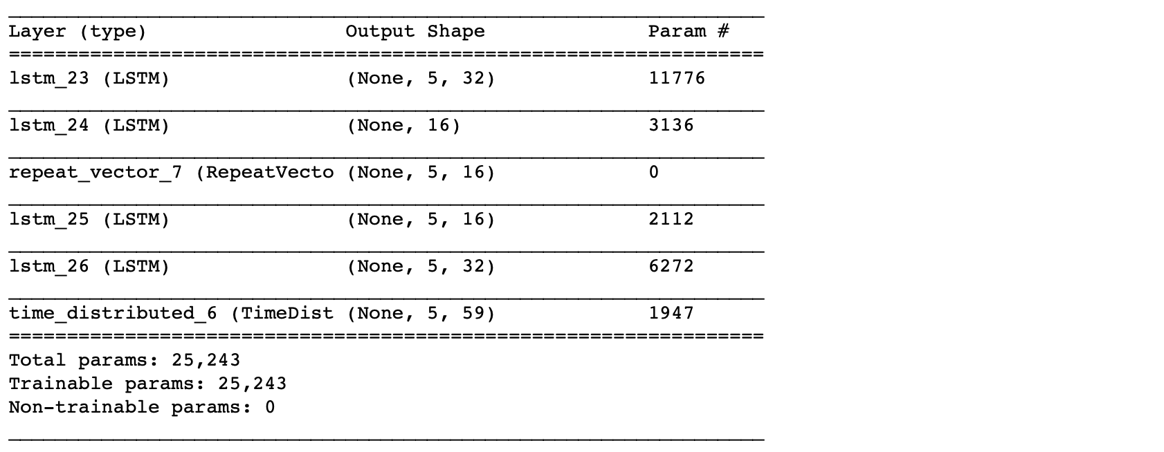
From the summary(), the total number of parameters are 5,331. This is about half of the training size. Hence, this is an appropriate model to fit. To have a bigger architecture, we will need to add regularization, e.g. Dropout, which will be covered in the next post.
Now, we will train the autoencoder.
adam = optimizers.Adam(lr)
lstm_autoencoder.compile(loss='mse', optimizer=adam)

cp = ModelCheckpoint(filepath="lstm_autoencoder_classifier.h5",
                               save_best_only=True,
                               verbose=0)

tb = TensorBoard(log_dir='./logs',
                histogram_freq=0,
                write_graph=True,
                write_images=True)

lstm_autoencoder_history = lstm_autoencoder.fit(X_train_y0_scaled, X_train_y0_scaled,
                                                epochs=epochs,
                                                batch_size=batch,
                                                validation_data=(X_valid_y0_scaled, X_valid_y0_scaled),
                                                verbose=2).history
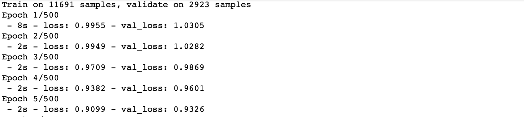
Plotting the change in the loss over the epochs.
plt.plot(lstm_autoencoder_history['loss'], linewidth=2, label='Train')
plt.plot(lstm_autoencoder_history['val_loss'], linewidth=2, label='Valid')
plt.legend(loc='upper right')
plt.title('Model loss')
plt.ylabel('Loss')
plt.xlabel('Epoch')
plt.show()
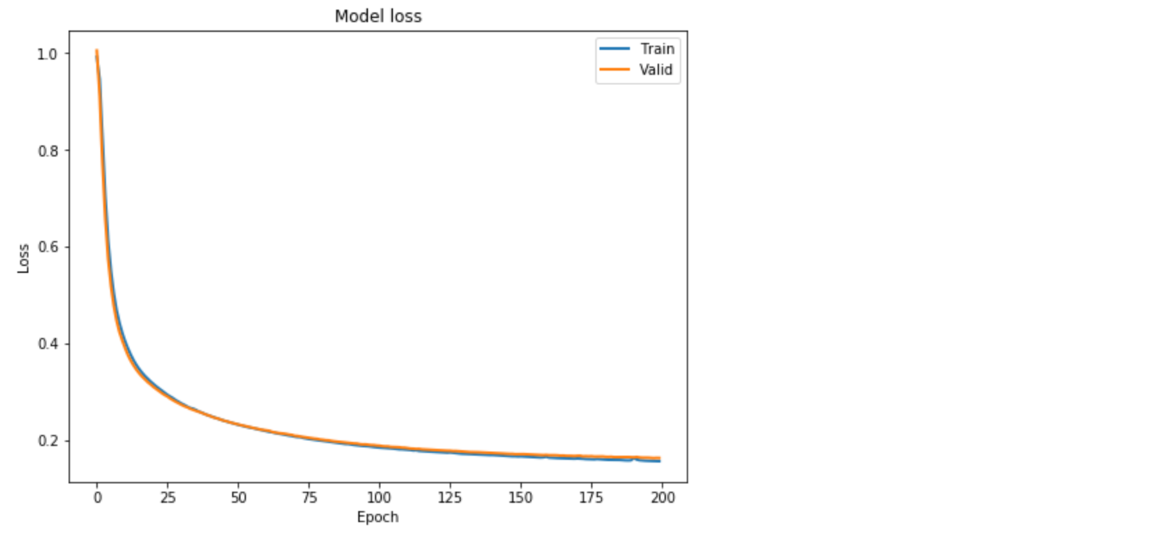
Figure 2. Loss function over the epochs.
Classification
Similar to the previous post [1], here we show how we can use an Autoencoder reconstruction error for the rare-event classification. We follow this concept: the autoencoder is expected to reconstruct a noif the reconstruction error is high, we will classify it as a sheet-break.
We will need to determine the threshold for this. Also, note that here we will be using the entire validation set containing both y = 0 or 1.
valid_x_predictions = lstm_autoencoder.predict(X_valid_scaled)
mse = np.mean(np.power(flatten(X_valid_scaled) - flatten(valid_x_predictions), 2), axis=1)

error_df = pd.DataFrame({'Reconstruction_error': mse,
                        'True_class': y_valid.tolist()})

precision_rt, recall_rt, threshold_rt = precision_recall_curve(error_df.True_class, error_df.Reconstruction_error)
plt.plot(threshold_rt, precision_rt[1:], label="Precision",linewidth=5)
plt.plot(threshold_rt, recall_rt[1:], label="Recall",linewidth=5)
plt.title('Precision and recall for different threshold values')
plt.xlabel('Threshold')
plt.ylabel('Precision/Recall')
plt.legend()
plt.show()
Note that we have to flatten the arrays to compute the mse.
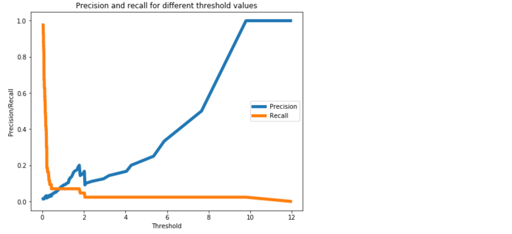
Figure 3. A threshold of 0.3 should provide a reasonable trade-off between precision and recall, as we want to higher recall.
Now, we will perform classification on the test data.
We should not estimate the classification threshold from the test data. It will result in overfitting.
test_x_predictions = lstm_autoencoder.predict(X_test_scaled)
mse = np.mean(np.power(flatten(X_test_scaled) - flatten(test_x_predictions), 2), axis=1)

error_df = pd.DataFrame({'Reconstruction_error': mse,
                        'True_class': y_test.tolist()})

threshold_fixed = 0.3
groups = error_df.groupby('True_class')
fig, ax = plt.subplots()

for name, group in groups:
    ax.plot(group.index, group.Reconstruction_error, marker='o', ms=3.5, linestyle='',
            label= "Break" if name == 1 else "Normal")
ax.hlines(threshold_fixed, ax.get_xlim()[0], ax.get_xlim()[1], colors="r", zorder=100, label='Threshold')
ax.legend()
plt.title("Reconstruction error for different classes")
plt.ylabel("Reconstruction error")
plt.xlabel("Data point index")
plt.show();
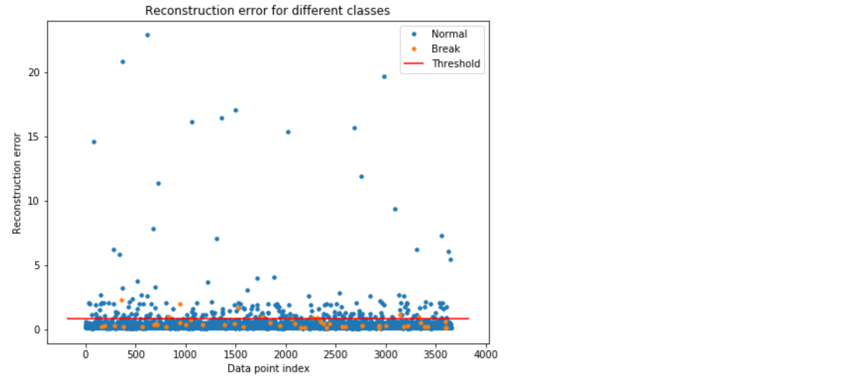
Figure 4. Using threshold = 0.8 for classification. The orange and blue dots above the threshold line represents the True Positive and False Positive, respectively.
In Figure 4, the orange and blue dot above the threshold line represents the True Positive and False Positive, respectively. As we can see, we have good number of false positives.
Let’s see the accuracy results.
Test Accuracy
Confusion Matrix
pred_y = [1 if e > threshold_fixed else 0 for e in error_df.Reconstruction_error.values]conf_matrix = confusion_matrix(error_df.True_class, pred_y)

plt.figure(figsize=(6, 6))
sns.heatmap(conf_matrix, xticklabels=LABELS, yticklabels=LABELS, annot=True, fmt="d");
plt.title("Confusion matrix")
plt.ylabel('True class')
plt.xlabel('Predicted class')
plt.show()
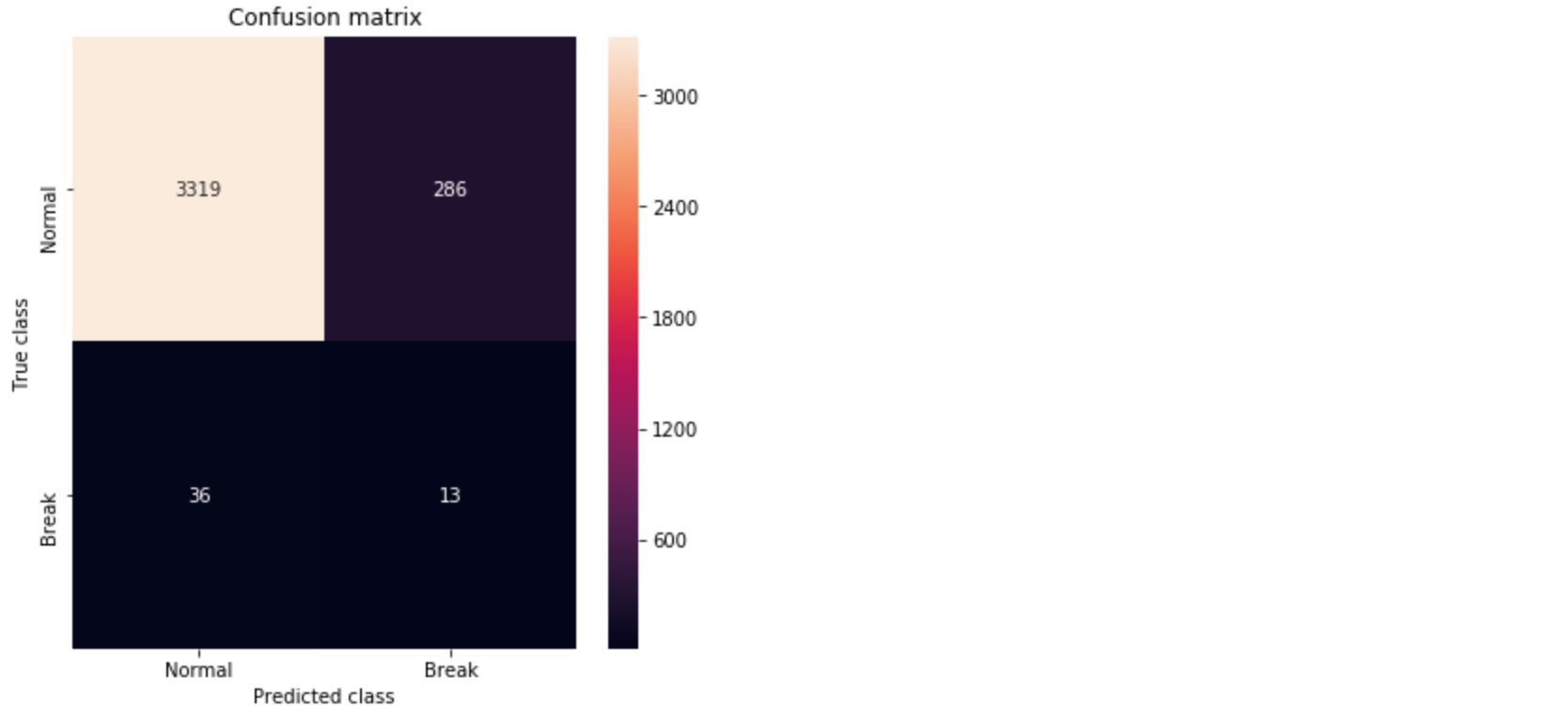
Figure 5. Confusion matrix showing the True Positives and False Positives.
ROC Curve and AUC
false_pos_rate, true_pos_rate, thresholds = roc_curve(error_df.True_class, error_df.Reconstruction_error)
roc_auc = auc(false_pos_rate, true_pos_rate,)

plt.plot(false_pos_rate, true_pos_rate, linewidth=5, label='AUC = %0.3f'% roc_auc)
plt.plot([0,1],[0,1], linewidth=5)

plt.xlim([-0.01, 1])
plt.ylim([0, 1.01])
plt.legend(loc='lower right')
plt.title('Receiver operating characteristic curve (ROC)')
plt.ylabel('True Positive Rate')
plt.xlabel('False Positive Rate')
plt.show()
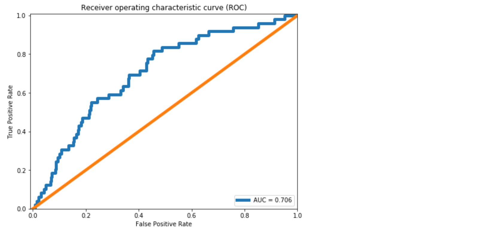
Figure 6. The ROC curve.
We see approximately 10% improvement in the AUC compared to the dense layer Autoencoder in [1]. From the Confusion Matrix in Figure 5, we could predict 10 out of 39 break instances. As also discussed in [1], this is significant for a paper mill. However, the improvement we achieved in comparison to the dense layer Autoencoder is minor.
The primary reason is LSTM model has more parameters to estimate. It becomes important to use regularization with LSTMs. Regularization and other model improvements will be discussed in the next post.
Github repository
cran2367/lstm_autoencoder_classifier
An LSTM Autoencoder for rare event classification. Contribute to cran2367/lstm_autoencoder_classifier development by…
github.com
What can be done better?
In the next article, we will learn tuning an Autoencoder. We will go over,
- CNN LSTM Autoencoder,
- Dropout layer,
- LSTM Dropout (Dropout_U and Dropout_W)
- Gaussian-dropout layer
- SELU activation, and
- alpha-dropout with SELU activation.
Conclusion
This post continued the work on extreme rare event binary labeled data in [1]. To utilize the temporal patterns, LSTM Autoencoders is used to build a rare event classifier for a multivariate time-series process. Details about the data preprocessing steps for LSTM model are discussed. A simple LSTM Autoencoder model is trained and used for classification. Some improvement in the accuracy over a Dense Autoencoder is found. For further improvement, we will look at ways to improve an Autoencoder with Dropout and other techniques in the next post.
Sequence embedding for clustering and classification
Here we will learn an approach to get vector embeddings for string sequences. These embeddings can be used for Clustering and Classification.
Sequence modeling has been a challenge. This is because of the inherent un-structuredness of sequence data. Just like texts in Natural Language Processing (NLP), sequences are arbitrary strings. For a computer, these strings have no meaning. As a result, building a data mining model is difficult.
For texts, we have come up with embeddings, such as word2vec, that convert a word into an n-dimensional vector. Essentially, bringing it in a Euclidean space. In this post, we will learn to do the same for sequences.
Here we will go over an approach to create embeddings for sequences that bring a sequence in a Euclidean space. With these embeddings, we can perform conventional Machine Learning and Deep Learning, e.g. K-means, PCA, and Multi-Layer Perceptron on sequence datasets. We provide and work on two datasets — protein sequences and weblogs.
Sequence datasets are commonly found around us. For example, clickstreams, music listening history, and weblogs in tech industries. In BioInformatics, we have large databases of protein sequences. A protein sequence is made of some combination of 20 amino acids. A typical protein sequence is shown where each letter corresponds to an amino acid.
A protein sequence does not necessarily contain all the 20 amino acids but some subset of it.
For clarity, we will define some keywords used in this post.
- alphabet: the discrete elements that make up a sequence. E.g. an amino acid.
- alphabet-set: a set of all alphabets that will make sequences in a corpus. E.g. all protein sequences in a corpus are made of a set of 20 amino acids.
- sequence: an ordered series of discrete alphabets. A sequence in a corpus contains a subset of alphabet-set.
The sequence corpus typically contains thousands to millions of sequences. Clustering and Classification are often required given we have labeled or unlabeled data. However, doing this is not straightforward due to the un-structuredness of sequences — arbitrary strings of arbitrary length.
To overcome this, sequence embeddings can be used. Here we will use an SGT embedding that embeds the long- and short- term patterns in a sequence into a finite-dimensional vector. The advantage of SGT embedding is that we can easily tune the amount of long- / short- term patterns without increasing the computation.
The source code and data in the following is here. Before moving forward, we will need to install Sgt package:
sgt
$ pip install sgt
Clustering
Protein Sequence Clustering
The data used here is taken from www.uniprot.org. This is a public database for proteins. The data contains the protein sequences and their function. In this section, we will cluster the protein sequences, and in the next we will use their functions as labels for building a classifier.
We first read the sequence data, and convert it into a list of lists. As shown below, each sequence is a list of alphabets.
>>> protein_data = pd.DataFrame.from_csv('../data/protein_classification.csv')
>>> X = protein_data['Sequence']
>>> def split(word):
>>>    return [char for char in word]>>> sequences = [split(x) for x in X]
>>> print(sequences[0])
['M', 'E', 'I', 'E', 'K', 'T', 'N', 'R', 'M', 'N', 'A', 'L', 'F', 'E', 'F', 'Y', 'A', 'A', 'L', 'L', 'T', 'D', 'K', 'Q', 'M', 'N', 'Y', 'I', 'E', 'L', 'Y', 'Y', 'A', 'D', 'D', 'Y', 'S', 'L', 'A', 'E', 'I', 'A', 'E', 'E', 'F', 'G', 'V', 'S', 'R', 'Q', 'A', 'V', 'Y', 'D', 'N', 'I', 'K', 'R', 'T', 'E', 'K', 'I', 'L', 'E', 'D', 'Y', 'E', 'M', 'K', 'L', 'H', 'M', 'Y', 'S', 'D', 'Y', 'I', 'V', 'R', 'S', 'Q', 'I', 'F', 'D', 'Q', 'I', 'L', 'E', 'R', 'Y', 'P', 'K', 'D', 'D', 'F', 'L', 'Q', 'E', 'Q', 'I', 'E', 'I', 'L', 'T', 'S', 'I', 'D', 'N', 'R', 'E']
Next, we generate the sequence embeddings.
>>> from sgt import Sgt
>>> sgt = Sgt(kappa = 10, lengthsensitive = False)
>>> embedding = sgt.fit_transform(corpus=sequences)
The embedding is in 400-dimensional space. Let’s first do PCA on it and reduce the dimension to two. This will also help visualize the clusters.
>>> pca = PCA(n_components=2)
>>> pca.fit(embedding)
>>> X = pca.transform(embedding)>>> print(np.sum(pca.explained_variance_ratio_))
0.6019403543806409
The top two PCs are explaining about 60% of the variance. We will cluster them into 3 clusters.
>>> kmeans = KMeans(n_clusters=3, max_iter =300)
>>> kmeans.fit(df)>>> labels = kmeans.predict(df)
>>> centroids = kmeans.cluster_centers_>>> fig = plt.figure(figsize=(5, 5))
>>> colmap = {1: 'r', 2: 'g', 3: 'b'}
>>> colors = list(map(lambda x: colmap[x+1], labels))
>>> plt.scatter(df['x1'], df['x2'], color=colors, alpha=0.5, edgecolor=colors)
Moving on to building classifiers.
Classification
Protein Sequence Classification
We will start by building a classifier on the same protein dataset we used earlier. The proteins in the dataset have two functions. Therefore, we will build a binary classifier.
We will first convert the:
function [CC]
a column in the data into labels that can be ingested in an MLP model built-in
keras
>>> y = protein_data['Function [CC]']
>>> encoder = LabelEncoder()
>>> encoder.fit(y)
>>> encoded_y = encoder.transform(y)
In the following, we build the MLP classifier and run 10-fold cross-validation.
>>> kfold = 10
>>> X = pd.DataFrame(embedding)
>>> y = encoded_y>>> random_state = 1>>> test_F1 = np.zeros(kfold)
>>> skf = KFold(n_splits = kfold, shuffle = True, random_state = random_state)
>>> k = 0
>>> epochs = 50
>>> batch_size = 128>>> for train_index, test_index in skf.split(X, y):
>>>     X_train, X_test = X.iloc[train_index], X.iloc[test_index]
>>>     y_train, y_test = y[train_index], y[test_index]
>>>     X_train = X_train.as_matrix(columns = None)
>>>     X_test = X_test.as_matrix(columns = None)
>>>
>>>     model = Sequential()
>>>     model.add(Dense(64, input_shape = (X_train.shape[1],), init = 'uniform'))
>>>     model.add(Activation('relu'))
>>>     model.add(Dropout(0.5))
>>>     model.add(Dense(32, init='uniform'))
>>>     model.add(Activation('relu'))
>>>     model.add(Dropout(0.5))
>>>     model.add(Dense(1, init='uniform'))
>>>     model.add(Activation('sigmoid'))
>>>     model.compile(loss='binary_crossentropy', optimizer='adam', metrics=['accuracy'])
>>>
>>>     model.fit(X_train, y_train ,batch_size=batch_size, epochs=epochs, verbose=0)
>>>
>>>     y_pred = model.predict_proba(X_test).round().astype(int)
>>>     y_train_pred = model.predict_proba(X_train).round().astype(int)>>>     test_F1[k] = sklearn.metrics.f1_score(y_test, y_pred)
>>>     k+=1

>>> print ('Average test f1-score', np.mean(test_F1))
Average test f1-score 1.0
This data turns out to be too good for the classifier. We have another dataset that is more challenging. Let’s go over it.
Network Log Data Classification
This data sample is taken from here. This is a network intrusion data containing audit logs and any attack as a positive label. Since network intrusion is a rare event, the data is unbalanced. Additionally, we have a small dataset of only 111 records. Here we will build a sequence classification model to predict a network intrusion.
Each sequence contains in the data is a series of activity, for example,
{login, password, …}
The alphabets in the input data sequences are already encoded into integers. The original sequences data file is present here.
Similar to before, we will first prepare the data for a classifier.
>>> darpa_data = pd.DataFrame.from_csv('../data/darpa_data.csv')
>>> X = darpa_data['seq']
>>> sequences = [x.split('~') for x in X]>>> y = darpa_data['class']
>>> encoder = LabelEncoder()
>>> encoder.fit(y)
>>> y = encoder.transform(y)
In this data, the sequence embeddings should be length-sensitive. The lengths are important here because sequences with similar patterns but different lengths can have different labels. Consider a simple example of two sessions:
{login, pswd, login, pswd,…}
{login, pswd,…(repeated several times)…, login, pswd}
While the first session can be a regular user mistyping the password once, the other session is possibly an attack to guess the password. Thus, the sequence lengths are as important as the patterns.
>>> sgt_darpa = Sgt(kappa = 5, lengthsensitive = True)
>>> embedding = sgt_darpa.fit_transform(corpus=sequences)
The embedding we find here is sparse. Therefore, we will perform dimension reduction using PCA before we train a classifier.
>>> from sklearn.decomposition import PCA
>>> pca = PCA(n_components=35)
>>> pca.fit(embedding)
>>> X = pca.transform(embedding)
>>> print(np.sum(pca.explained_variance_ratio_))
0.9862350164327149
The selected top-35 PCAs are explaining more than 98% of the variance. We will now go ahead and build a Multi-Layer Perceptron using keras. Since the data size is small and, also, the number of positive labeled points, we will perform a 3-fold validation.
>>> kfold = 3
>>> random_state = 11>>> test_F1 = np.zeros(kfold)
>>> time_k = np.zeros(kfold)
>>> skf = StratifiedKFold(n_splits=kfold, shuffle=True, random_state=random_state)
>>> k = 0
>>> epochs = 300
>>> batch_size = 15>>> class_weight = {0 : 0.12, 1: 0.88,}  # The weights can be changed and made inversely proportional to the class size to improve the accuracy.>>> for train_index, test_index in skf.split(X, y):
>>>     X_train, X_test = X[train_index], X[test_index]
>>>     y_train, y_test = y[train_index], y[test_index]
>>>
>>>     model = Sequential()
>>>     model.add(Dense(128, input_shape=(X_train.shape[1],), init='uniform'))
>>>     model.add(Activation('relu'))
>>>     model.add(Dropout(0.5))
>>>     model.add(Dense(1, init='uniform'))
>>>     model.add(Activation('sigmoid'))
>>>     model.summary()
>>>     model.compile(loss='binary_crossentropy', optimizer='adam', metrics=['accuracy'])
>>>
>>>     start_time = time.time()
>>>     model.fit(X_train, y_train ,batch_size=batch_size, epochs=epochs, verbose=1, class_weight=class_weight)
>>>     end_time = time.time()
>>>     time_k[k] = end_time-start_time>>>     y_pred = model.predict_proba(X_test).round().astype(int)
>>>     y_train_pred = model.predict_proba(X_train).round().astype(int)
>>>     test_F1[k] = sklearn.metrics.f1_score(y_test, y_pred)
>>>     k += 1
>>> print ('Average Test f1-score', np.mean(test_F1))
Average Test f1-score 0.5236467236467236>>> print ('Average Run time', np.mean(time_k))
Average Run time 9.076935768127441
This was a difficult data to classify. To have a loose benchmark, let’s build a fancier LSTM classifier on the same data.
>>> X = darpa_data['seq']
>>> encoded_X = np.ndarray(shape=(len(X),), dtype=list)
>>> for i in range(0,len(X)):
>>>     encoded_X[i]=X.iloc[i].split("~")
>>> max_seq_length = np.max(darpa_data['seqlen'])
>>> encoded_X = sequence.pad_sequences(encoded_X, maxlen=max_seq_length)>>> kfold = 3
>>> random_state = 11>>> test_F1 = np.zeros(kfold)
>>> time_k = np.zeros(kfold)>>> epochs = 50
>>> batch_size = 15
>>> skf = StratifiedKFold(n_splits=kfold, shuffle=True, random_state=random_state)
>>> k = 0>>> for train_index, test_index in skf.split(encoded_X, y):
>>>     X_train, X_test = encoded_X[train_index], encoded_X[test_index]
>>>     y_train, y_test = y[train_index], y[test_index]
>>>
>>>     embedding_vecor_length = 32
>>>     top_words=50
>>>     model = Sequential()
>>>     model.add(Embedding(top_words, embedding_vecor_length, input_length=max_seq_length))
>>>     model.add(LSTM(32))
>>>     model.add(Dense(1, init='uniform'))
>>>     model.add(Activation('sigmoid'))
>>>     model.compile(loss='binary_crossentropy', optimizer='adam', metrics=['accuracy'])>>>     start_time = time.time()
>>>     model.fit(X_train, y_train, epochs=epochs, batch_size=batch_size, verbose=1)
>>>     end_time=time.time()
>>>     time_k[k]=end_time-start_time>>>     y_pred = model.predict_proba(X_test).round().astype(int)
>>>     y_train_pred=model.predict_proba(X_train).round().astype(int)
>>>     test_F1[k]=sklearn.metrics.f1_score(y_test, y_pred)
>>>     k+=1>>> print ('Average Test f1-score', np.mean(test_F1))
Average Test f1-score 0.0>>> print ('Average Run time', np.mean(time_k))
Average Run time 425.68603706359863
We find that the LSTM classifier gives an F1 score of 0. This may be improved by changing the model. However, we find that the SGT embedding could work with small and unbalanced data without the need of a complicated classifier. Besides, on the runtime, SGT embedded network was significantly faster. It took on average 9.1 secs while the LSTM model took 425.6 secs.
Concluding Remarks
- We learned about using a sequence embedding for sequence clustering and classification.
- This embedding is an implementation of this paper. Not covered in this post, but refer to this paper to see the accuracy comparison of SGT embedding over others.
- Due to SGT embedding’s ability to capture long- and short- term patterns, it works better than most other sequence modeling approaches.
- It is recommended that you play with the tuning parameter, kappa, to see its effect on accuracy.
Related Articles
Estimating non-linear correlation in R
In this post, we will learn about using a nonlinear correlation estimation function in R. We will also look at a few examples.
Background
Correlation estimations are commonly used in various data mining applications. In my experience, nonlinear correlations are quite common in various processes. Due to this, nonlinear models, such as SVM, are employed for regression, classification, etc. However, there are not many approaches to estimate nonlinear correlations between two variables.
Typically linear correlations are estimated. However, the data may have a nonlinear correlation but little to no linear correlation. In such cases, nonlinearly correlated variables are sometimes overlooked during data exploration or variable selection in high-dimensional data.
We have developed a new nonlinear correlation estimator:
nlcor
This estimator comes useful in data exploration and also variable selection for nonlinear predictive models, such as SVM.
Installing
To install
nlcor
in R, follow these steps:
- Install the devtools package. You can do this from CRAN. You can do it directly in R console by typing,
> install.packages("devtools")
2. Load the devtools package.
> library(devtools)
3. Install
nlcor
from its GitHub repository by typing this in R console.
> install_github("ProcessMiner/nlcor")
Nonlinear Correlation Estimator: Nlcor
In this package, we provide an implementation of a nonlinear correlation estimation method using an adaptive local linear correlation computation in
nlcor
The function
nlcor
returns the nonlinear correlation estimate, the corresponding adjusted p-value, and an optional plot visualizing the nonlinear relationships.
The correlation estimate will be between 0 and 1. The higher the value the more is the nonlinear correlation. Unlike linear correlations, a negative value is not valid here. Due to multiple local correlation computations, the net p-value of the correlation estimate is adjusted (to avoid false positives). The plot visualizes the local linear correlations.
In the following, we will show its usage with a few examples. In the given examples, the linear correlations between
x
and
nlcor
is small, however, there is a visible nonlinear correlation between them. This package contains the data for these examples and can be used for testing the package.
nlcor
package has few sample
x
and
y
vectors that are demonstrated in the following examples.
First, we will load the package.
> library(nlcor)
Example 1. A data with cyclic nonlinear correlation.
> plot(x1, y1)
The linear correlation of the data is,
> cor(x1, y1)
[1] 0.008001837
As expected, the correlation is close to zero. We estimate the nonlinear correlation using
nlcor
> c <- nlcor(x1, y1, plt = T)
> c$cor.estimate
[1] 0.8688784
> c$adjusted.p.value
[1] 0
> print(c$cor.plot)
The plot shows the piecewise linear correlations present in the data.
Example 2. A data with non-uniform piecewise linear correlations.
> plot(x2, y2)
The linear correlation of the data is,
> cor(x2, y2)
[1] 0.828596
The linear correlation is quite high in this data. However, there is significant and higher nonlinear correlation present in the data. This data emulates the scenario where the correlation changes its direction after a point. Sometimes that change point is in the middle causing the linear correlation to be close to zero. Here we show an example when the change point is off-center to show that the implementation works in non-uniform cases.
We estimate the nonlinear correlation using
nlcor
> c <- nlcor(x2, y2, plt = T)
> c$cor.estimate
[1] 0.897205
> c$adjusted.p.value
[1] 0
> print(c$cor.plot)
It is visible from the plot that
nlcor
could estimate the piecewise correlations in a non-uniform scenario. Also, the nonlinear correlation comes out to be higher than the linear correlation.
Example 3. A data with higher and multiple frequency variations.
> plot(x3, y3)
The linear correlation of the data is,
> cor(x3, y3)
[1] -0.1337304
The linear correlation is expectedly small, albeit not close to zero due to some linearity.
Here we show we can refine the granularity of the correlation computation.
Under default settings, the output of
nlcor
will be
> c <- nlcor(x3, y3, plt = T)
> c$cor.estimate
[1] 0.7090148
> c$adjusted.p.value
[1] 0
> print(c$cor.plot)
As can be seen in the figure,
nlcor
could identify the granular piecewise correlations. In this data, the p-value still remains extremely small—the correlation is statistically significant.
Summary
This package provides an implementation of an efficient heuristic to compute the nonlinear correlations between numeric vectors. The heuristic works by adaptively identifying multiple local regions of linear correlations to estimate the overall nonlinear correlation. Its usages are demonstrated here with few examples.