Here we will learn an approach to get vector embeddings for string sequences. These embeddings can be used for Clustering and Classification.
Sequence modeling has been a challenge. This is because of the inherent un-structuredness of sequence data. Just like texts in Natural Language Processing (NLP), sequences are arbitrary strings. For a computer, these strings have no meaning. As a result, building a data mining model is difficult.
For texts, we have come up with embeddings, such as word2vec, that convert a word into an n-dimensional vector. Essentially, bringing it in a Euclidean space. In this post, we will learn to do the same for sequences.
Here we will go over an approach to create embeddings for sequences that bring a sequence in a Euclidean space. With these embeddings, we can perform conventional Machine Learning and Deep Learning, e.g. K-means, PCA, and Multi-Layer Perceptron on sequence datasets. We provide and work on two datasets — protein sequences and weblogs.
Sequence datasets are commonly found around us. For example, clickstreams, music listening history, and weblogs in tech industries. In BioInformatics, we have large databases of protein sequences. A protein sequence is made of some combination of 20 amino acids. A typical protein sequence is shown where each letter corresponds to an amino acid.
A protein sequence does not necessarily contain all the 20 amino acids but some subset of it.
For clarity, we will define some keywords used in this post.
- alphabet: the discrete elements that make up a sequence. E.g. an amino acid.
- alphabet-set: a set of all alphabets that will make sequences in a corpus. E.g. all protein sequences in a corpus are made of a set of 20 amino acids.
- sequence: an ordered series of discrete alphabets. A sequence in a corpus contains a subset of alphabet-set.
The sequence corpus typically contains thousands to millions of sequences. Clustering and Classification are often required given we have labeled or unlabeled data. However, doing this is not straightforward due to the un-structuredness of sequences — arbitrary strings of arbitrary length.
To overcome this, sequence embeddings can be used. Here we will use an SGT embedding that embeds the long- and short- term patterns in a sequence into a finite-dimensional vector. The advantage of SGT embedding is that we can easily tune the amount of long- / short- term patterns without increasing the computation.
The source code and data in the following is here. Before moving forward, we will need to install Sgt package:
sgt
$ pip install sgt
Clustering
Protein Sequence Clustering
The data used here is taken from www.uniprot.org. This is a public database for proteins. The data contains the protein sequences and their function. In this section, we will cluster the protein sequences, and in the next we will use their functions as labels for building a classifier.
We first read the sequence data, and convert it into a list of lists. As shown below, each sequence is a list of alphabets.
>>> protein_data = pd.DataFrame.from_csv('../data/protein_classification.csv')
>>> X = protein_data['Sequence']
>>> def split(word):
>>>    return [char for char in word]>>> sequences = [split(x) for x in X]
>>> print(sequences[0])
['M', 'E', 'I', 'E', 'K', 'T', 'N', 'R', 'M', 'N', 'A', 'L', 'F', 'E', 'F', 'Y', 'A', 'A', 'L', 'L', 'T', 'D', 'K', 'Q', 'M', 'N', 'Y', 'I', 'E', 'L', 'Y', 'Y', 'A', 'D', 'D', 'Y', 'S', 'L', 'A', 'E', 'I', 'A', 'E', 'E', 'F', 'G', 'V', 'S', 'R', 'Q', 'A', 'V', 'Y', 'D', 'N', 'I', 'K', 'R', 'T', 'E', 'K', 'I', 'L', 'E', 'D', 'Y', 'E', 'M', 'K', 'L', 'H', 'M', 'Y', 'S', 'D', 'Y', 'I', 'V', 'R', 'S', 'Q', 'I', 'F', 'D', 'Q', 'I', 'L', 'E', 'R', 'Y', 'P', 'K', 'D', 'D', 'F', 'L', 'Q', 'E', 'Q', 'I', 'E', 'I', 'L', 'T', 'S', 'I', 'D', 'N', 'R', 'E']
Next, we generate the sequence embeddings.
>>> from sgt import Sgt
>>> sgt = Sgt(kappa = 10, lengthsensitive = False)
>>> embedding = sgt.fit_transform(corpus=sequences)
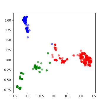
The embedding is in 400-dimensional space. Let’s first do PCA on it and reduce the dimension to two. This will also help visualize the clusters.
>>> pca = PCA(n_components=2)
>>> pca.fit(embedding)
>>> X = pca.transform(embedding)>>> print(np.sum(pca.explained_variance_ratio_))
0.6019403543806409
The top two PCs are explaining about 60% of the variance. We will cluster them into 3 clusters.
>>> kmeans = KMeans(n_clusters=3, max_iter =300)
>>> kmeans.fit(df)>>> labels = kmeans.predict(df)
>>> centroids = kmeans.cluster_centers_>>> fig = plt.figure(figsize=(5, 5))
>>> colmap = {1: 'r', 2: 'g', 3: 'b'}
>>> colors = list(map(lambda x: colmap[x+1], labels))
>>> plt.scatter(df['x1'], df['x2'], color=colors, alpha=0.5, edgecolor=colors)
Moving on to building classifiers.
Classification
Protein Sequence Classification
We will start by building a classifier on the same protein dataset we used earlier. The proteins in the dataset have two functions. Therefore, we will build a binary classifier.
We will first convert the:
function [CC]a column in the data into labels that can be ingested in an MLP model built-in
keras>>> y = protein_data['Function [CC]']
>>> encoder = LabelEncoder()
>>> encoder.fit(y)
>>> encoded_y = encoder.transform(y)In the following, we build the MLP classifier and run 10-fold cross-validation.
>>> kfold = 10
>>> X = pd.DataFrame(embedding)
>>> y = encoded_y>>> random_state = 1>>> test_F1 = np.zeros(kfold)
>>> skf = KFold(n_splits = kfold, shuffle = True, random_state = random_state)
>>> k = 0
>>> epochs = 50
>>> batch_size = 128>>> for train_index, test_index in skf.split(X, y):
>>>     X_train, X_test = X.iloc[train_index], X.iloc[test_index]
>>>     y_train, y_test = y[train_index], y[test_index]
>>>     X_train = X_train.as_matrix(columns = None)
>>>     X_test = X_test.as_matrix(columns = None)
>>>
>>>     model = Sequential()
>>>     model.add(Dense(64, input_shape = (X_train.shape[1],), init = 'uniform'))
>>>     model.add(Activation('relu'))
>>>     model.add(Dropout(0.5))
>>>     model.add(Dense(32, init='uniform'))
>>>     model.add(Activation('relu'))
>>>     model.add(Dropout(0.5))
>>>     model.add(Dense(1, init='uniform'))
>>>     model.add(Activation('sigmoid'))
>>>     model.compile(loss='binary_crossentropy', optimizer='adam', metrics=['accuracy'])
>>>
>>>     model.fit(X_train, y_train ,batch_size=batch_size, epochs=epochs, verbose=0)
>>>
>>>     y_pred = model.predict_proba(X_test).round().astype(int)
>>>     y_train_pred = model.predict_proba(X_train).round().astype(int)>>>     test_F1[k] = sklearn.metrics.f1_score(y_test, y_pred)
>>>     k+=1

>>> print ('Average test f1-score', np.mean(test_F1))
Average test f1-score 1.0
This data turns out to be too good for the classifier. We have another dataset that is more challenging. Let’s go over it.
Network Log Data Classification
This data sample is taken from here. This is a network intrusion data containing audit logs and any attack as a positive label. Since network intrusion is a rare event, the data is unbalanced. Additionally, we have a small dataset of only 111 records. Here we will build a sequence classification model to predict a network intrusion.
Each sequence contains in the data is a series of activity, for example,
{login, password, …}The alphabets in the input data sequences are already encoded into integers. The original sequences data file is present here.
Similar to before, we will first prepare the data for a classifier.
>>> darpa_data = pd.DataFrame.from_csv('../data/darpa_data.csv')
>>> X = darpa_data['seq']
>>> sequences = [x.split('~') for x in X]>>> y = darpa_data['class']
>>> encoder = LabelEncoder()
>>> encoder.fit(y)
>>> y = encoder.transform(y)
In this data, the sequence embeddings should be length-sensitive. The lengths are important here because sequences with similar patterns but different lengths can have different labels. Consider a simple example of two sessions:
{login, pswd, login, pswd,…}
{login, pswd,…(repeated several times)…, login, pswd}
While the first session can be a regular user mistyping the password once, the other session is possibly an attack to guess the password. Thus, the sequence lengths are as important as the patterns.
>>> sgt_darpa = Sgt(kappa = 5, lengthsensitive = True)
>>> embedding = sgt_darpa.fit_transform(corpus=sequences)
The embedding we find here is sparse. Therefore, we will perform dimension reduction using PCA before we train a classifier.
>>> from sklearn.decomposition import PCA
>>> pca = PCA(n_components=35)
>>> pca.fit(embedding)
>>> X = pca.transform(embedding)
>>> print(np.sum(pca.explained_variance_ratio_))
0.9862350164327149
The selected top-35 PCAs are explaining more than 98% of the variance. We will now go ahead and build a Multi-Layer Perceptron using keras. Since the data size is small and, also, the number of positive labeled points, we will perform a 3-fold validation.
>>> kfold = 3
>>> random_state = 11>>> test_F1 = np.zeros(kfold)
>>> time_k = np.zeros(kfold)
>>> skf = StratifiedKFold(n_splits=kfold, shuffle=True, random_state=random_state)
>>> k = 0
>>> epochs = 300
>>> batch_size = 15>>> class_weight = {0 : 0.12, 1: 0.88,}  # The weights can be changed and made inversely proportional to the class size to improve the accuracy.>>> for train_index, test_index in skf.split(X, y):
>>>     X_train, X_test = X[train_index], X[test_index]
>>>     y_train, y_test = y[train_index], y[test_index]
>>>
>>>     model = Sequential()
>>>     model.add(Dense(128, input_shape=(X_train.shape[1],), init='uniform'))
>>>     model.add(Activation('relu'))
>>>     model.add(Dropout(0.5))
>>>     model.add(Dense(1, init='uniform'))
>>>     model.add(Activation('sigmoid'))
>>>     model.summary()
>>>     model.compile(loss='binary_crossentropy', optimizer='adam', metrics=['accuracy'])
>>>
>>>     start_time = time.time()
>>>     model.fit(X_train, y_train ,batch_size=batch_size, epochs=epochs, verbose=1, class_weight=class_weight)
>>>     end_time = time.time()
>>>     time_k[k] = end_time-start_time>>>     y_pred = model.predict_proba(X_test).round().astype(int)
>>>     y_train_pred = model.predict_proba(X_train).round().astype(int)
>>>     test_F1[k] = sklearn.metrics.f1_score(y_test, y_pred)
>>>     k += 1
>>> print ('Average Test f1-score', np.mean(test_F1))
Average Test f1-score 0.5236467236467236>>> print ('Average Run time', np.mean(time_k))
Average Run time 9.076935768127441
This was a difficult data to classify. To have a loose benchmark, let’s build a fancier LSTM classifier on the same data.
>>> X = darpa_data['seq']
>>> encoded_X = np.ndarray(shape=(len(X),), dtype=list)
>>> for i in range(0,len(X)):
>>>     encoded_X[i]=X.iloc[i].split("~")
>>> max_seq_length = np.max(darpa_data['seqlen'])
>>> encoded_X = sequence.pad_sequences(encoded_X, maxlen=max_seq_length)>>> kfold = 3
>>> random_state = 11>>> test_F1 = np.zeros(kfold)
>>> time_k = np.zeros(kfold)>>> epochs = 50
>>> batch_size = 15
>>> skf = StratifiedKFold(n_splits=kfold, shuffle=True, random_state=random_state)
>>> k = 0>>> for train_index, test_index in skf.split(encoded_X, y):
>>>     X_train, X_test = encoded_X[train_index], encoded_X[test_index]
>>>     y_train, y_test = y[train_index], y[test_index]
>>>
>>>     embedding_vecor_length = 32
>>>     top_words=50
>>>     model = Sequential()
>>>     model.add(Embedding(top_words, embedding_vecor_length, input_length=max_seq_length))
>>>     model.add(LSTM(32))
>>>     model.add(Dense(1, init='uniform'))
>>>     model.add(Activation('sigmoid'))
>>>     model.compile(loss='binary_crossentropy', optimizer='adam', metrics=['accuracy'])>>>     start_time = time.time()
>>>     model.fit(X_train, y_train, epochs=epochs, batch_size=batch_size, verbose=1)
>>>     end_time=time.time()
>>>     time_k[k]=end_time-start_time>>>     y_pred = model.predict_proba(X_test).round().astype(int)
>>>     y_train_pred=model.predict_proba(X_train).round().astype(int)
>>>     test_F1[k]=sklearn.metrics.f1_score(y_test, y_pred)
>>>     k+=1>>> print ('Average Test f1-score', np.mean(test_F1))
Average Test f1-score 0.0>>> print ('Average Run time', np.mean(time_k))
Average Run time 425.68603706359863
We find that the LSTM classifier gives an F1 score of 0. This may be improved by changing the model. However, we find that the SGT embedding could work with small and unbalanced data without the need of a complicated classifier. Besides, on the runtime, SGT embedded network was significantly faster. It took on average 9.1 secs while the LSTM model took 425.6 secs.
Concluding Remarks
- We learned about using a sequence embedding for sequence clustering and classification.
- This embedding is an implementation of this paper. Not covered in this post, but refer to this paper to see the accuracy comparison of SGT embedding over others.
- Due to SGT embedding’s ability to capture long- and short- term patterns, it works better than most other sequence modeling approaches.
- It is recommended that you play with the tuning parameter, kappa, to see its effect on accuracy.
Related Articles
How Board Producer Reduced Chemistry Consumption by 14%
ProcessMiner Delivers 25% Reduction in Wet Strength Chemistry Usage
How Board Mill Optimizes Kymene Consumption
ProcessMiner Delivers 25% Reduction in Wet Strength Chemistry Usage
How Tissue & Towel Manufacturer Reduced Chemistry Use by 25%
ProcessMiner Delivers 25% Reduction in Wet Strength Chemistry Usage


